Chapter 4 Analysis

4.1 National Overview

In addition to the 10 focal states selected by Pew for this report, we ran the same metrics for all coastal states from the contiguous United States and the District of Columbia (Figure 4.1, Figure 4.2). In the context of all contiguous coastal U.S. states Massachusetts consistently ranked in the upper quartile of all metrics. Oregon, Louisiana, Washington, Delaware and California all ranked highly across multiple metrics. Regarding Oregon, it is important to understand that the area of seagrasses versus kelp beds could not be separated in the underlying mapping product and kelp beds can be extensive in this region. We consider the states of Massachusetts and Oregon to be our highest tier (tier 1).

The second tier of states are LA, WA, DE, and CA (total scores just below “best”) which scored well but can improve in one or two categories. LA scores well in spatial representativeness due to the CRMS network that dominates the database and was explicitly designed as a state-wide, spatially explicit sampling strategy. Despite this LA has fewer cores per 1,000 ha of wetlands because of the large area of tidal wetlands in the Mississippi River delta. The high score for LA means that the largest fraction of Blue Carbon ecosystems in CONUS – those of Mississippi River Delta – have some of the best soil carbon data available in the U.S. TX and AL are squarely in our second tier of states (i.e. total scores better than fair but below tier 1), leaving MS as the only Gulf coast state needing significant improvement in Blue Carbon data.

The third tier of states are FL, NJ, TX, NY, AL, SC, MD, and CT with total metric scores better than fair. The fourth tier of states are GA, NC and NH with total scores of fair, and the fifth tier are states with total scores below fair (RI, MS, VA, ME, PA and DC). PA and DC have mapped tidal wetlands, but do not have any soils data in our library, and it is not known if any data collection efforts are slated for entry (Figure 4.3).

Of the Atlantic coast states only DE was represented in the second-tier states because of the active contributions made by Brandon Boyd (US Army Corps of Engineers) and Kari St. Laurent (Delaware National Estuarine Research Reserve). Though DE holds a small proportion of CONUS coastal area, it is well-positioned in terms of data for Blue Carbon activities. CT, FL, SC, NJ, and NY on the Atlantic coast fell into our third tier. Other than MS, all of the states that fell into our lowest tier are on the Atlantic coast.

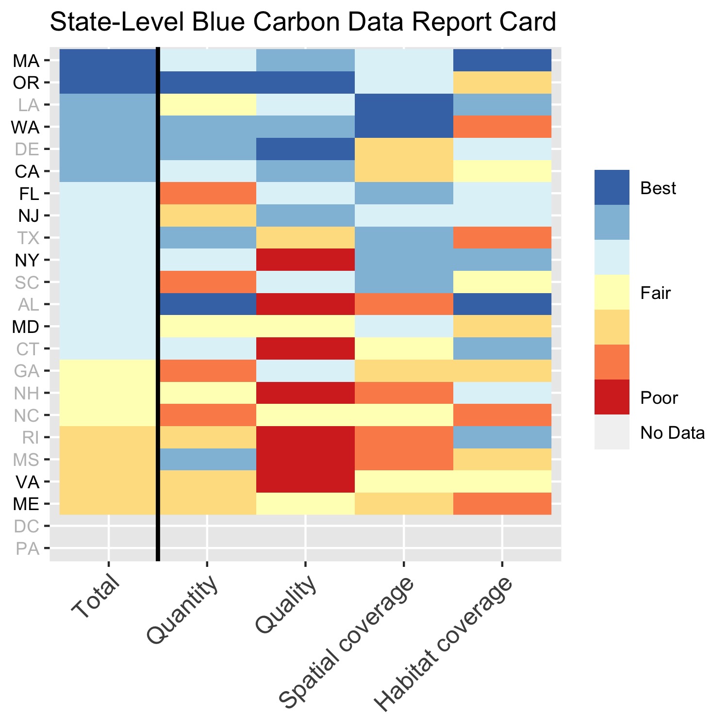
Figure 4.1: State Level Report Card showing rankings of all coastal states and the District of Columbia along four metrics: quantity, quality, spatial coverage and habitat coverage for focal states selected by Pew (black) and other coastal states in CONUS (grey). They are ordered top to bottom by their composite rank, calculated as the average of the other four rankings.

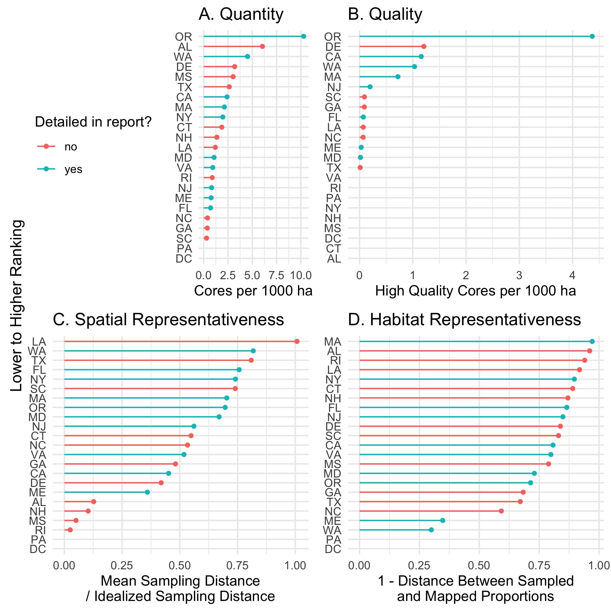
Figure 4.2: Magnitudes and rankings of all four metrics. All coastal states for all metrics are ranked from top to bottom, higher to lower ranking. A: Quantity, B. Quality, C. Spatial Representativeness, and D. Habitat Representativeness. Blue lines and symbols are the focal states for this report. Note that while A, B, and C rank best to worst as highest to lowest scoring, D. ranks best to worst as lowest to highest scoring.

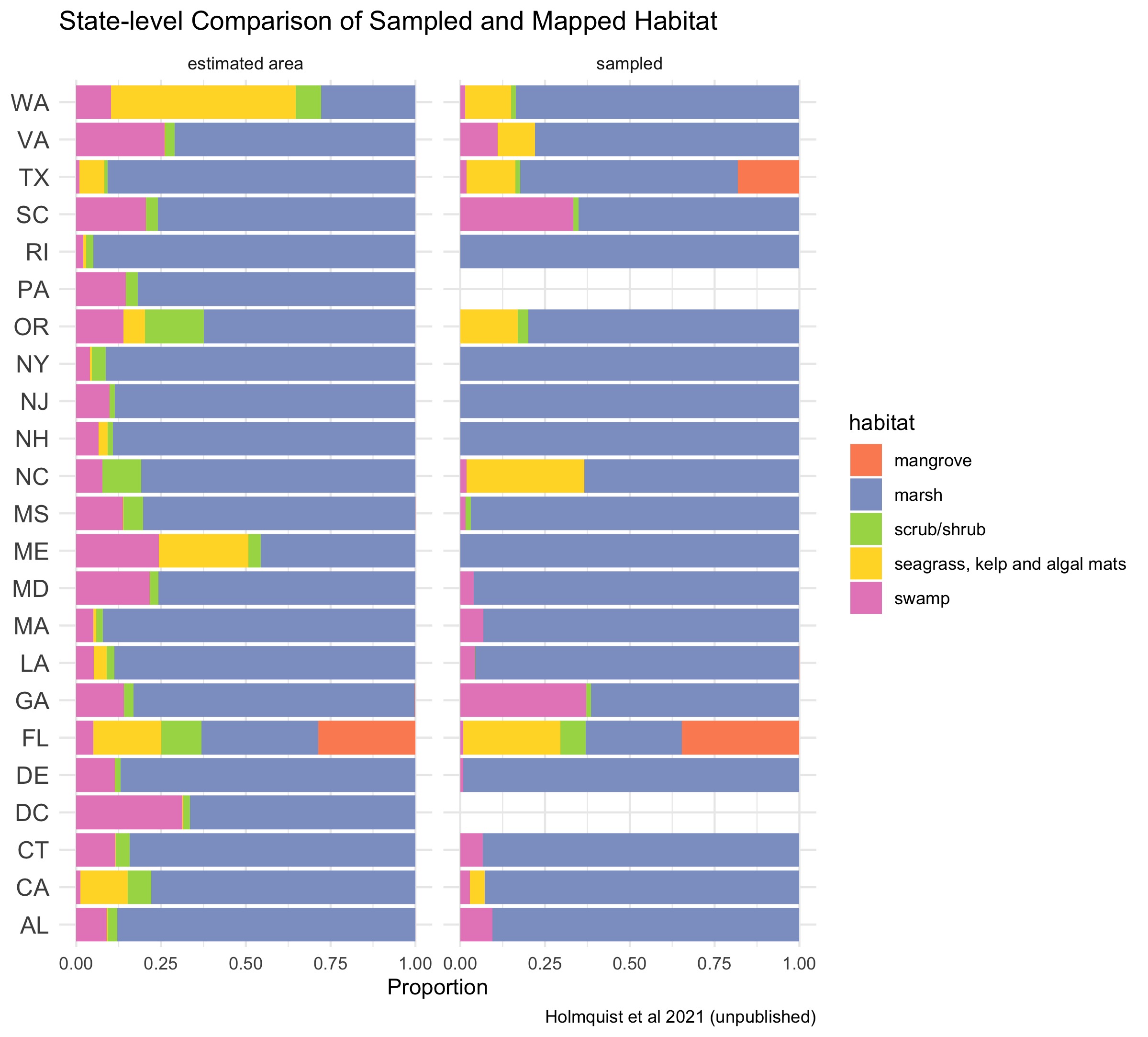
Figure 4.3: Proportions of various Blue Carbon habitats represented in the dataset in proportion to their estimated area. Seagrasses, kelp beds and algal mats are all combined into a single category, because they are combined in the underlying mapping products.

4.2 Overview of Blue Carbon Data in Pew-Selected States

Pew identified a subset of states with attributes that make them potentially attractive for climate mitigation projects in Blue Carbon ecosystems, namely California, Florida, Maine, Maryland, Massachusetts, New Jersey, New York, Oregon, Virginia, and Washington. We developed four new metrics that synthesize key features of the Coastal Carbon Atlas and are broadly relevant to management activities. Data quantity is the number of soil profiles available in the Atlas per 1,000 hectares of Blue Carbon habitat; data quality captures amount of data available for advanced use cases ranging from full profile carbon stock inventorying to carbon sequestration modeling (also expressed relative to Blue Carbon habitat area); spatial representativeness considers whether the observations are well distributed across the coastal geography of the state; and habitat representativeness does the same for habitat types found in a given state. The average of these provided a composite score.

4.3 California State Report

4.3.1 State Overview

The Coastal Carbon Atlas contains 139 cores from California or 3.7% of the cores sampled in CONUS. The quantity of soil cores available for California compared to those in the other coastal states is fairly representative of California’s contribution to the total U.S. coastal wetland area (Figure 4.4A, Figure 4.5). The soil core data of this state is relatively high quality, but falls below the median for spatial and habitat coverage (Figure 4.4). Improvements can be made to this state’s score through targeted sampling efforts aimed at increasing spatial and habitat representativeness.

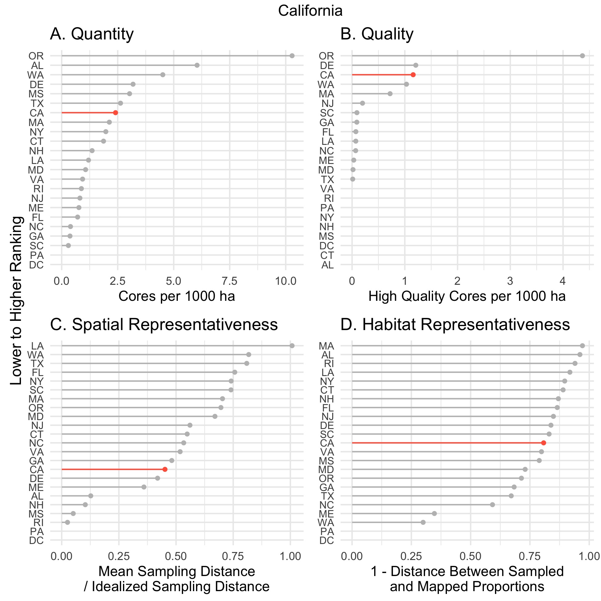
Figure 4.4: State ranking on all four soil Blue Carbon metrics, A. Quantity, B. Quality, C. Spatial Representativeness, D. Habitat Representativeness.

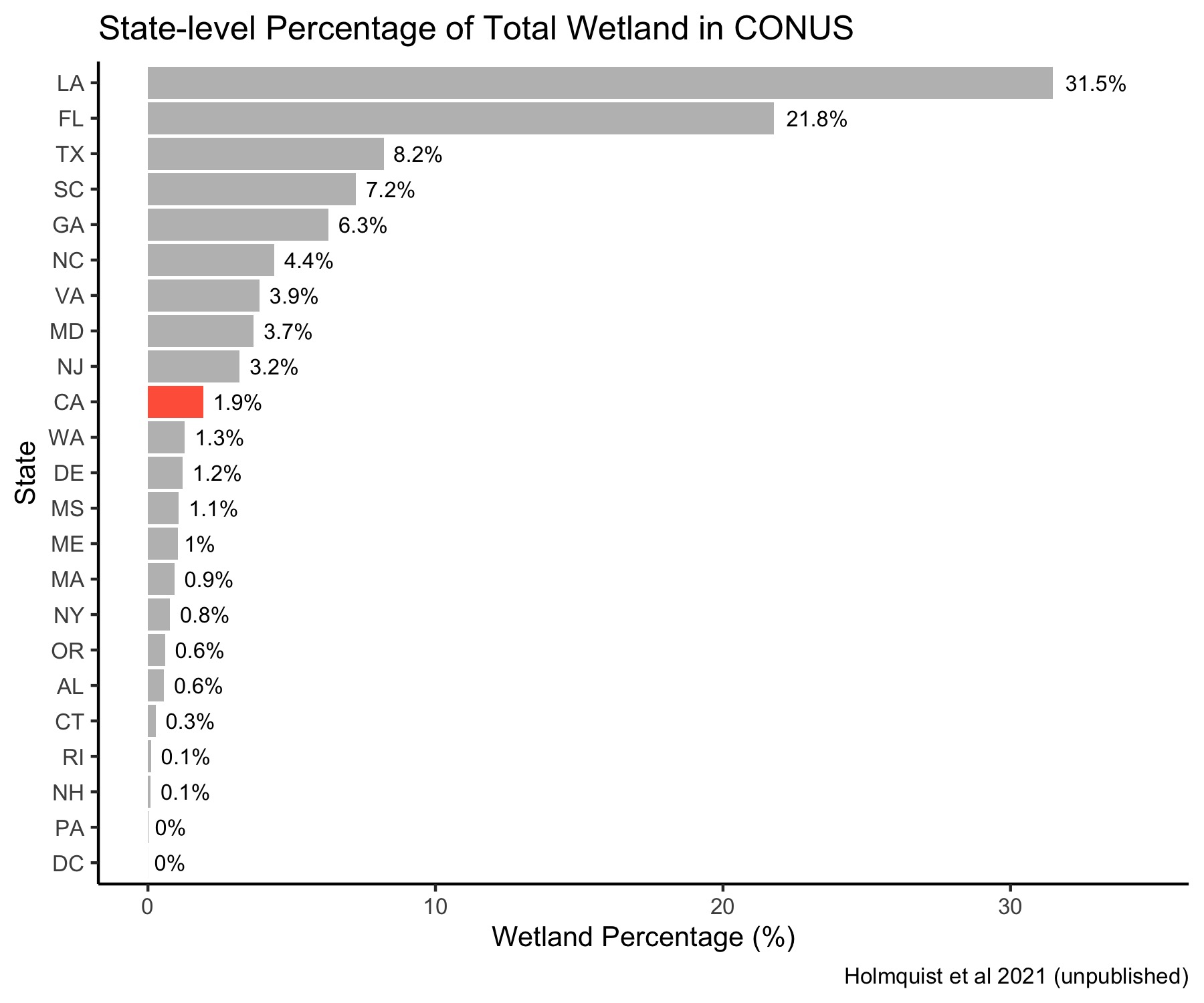
Figure 4.5: California State-Level Wetland Contribution

4.3.2 Data Utility and Availability

The data quality of the soil cores from California is high compared to other states (Figure 4.4B). All of this state’s cores possess information that is sufficient for carbon stock assessments, 64 of the cores can be used for carbon accretion rate assessments, and 43 of the cores have high-quality elevation data that is applicable for carbon sequestration modeling (Figure 4.6, Table 4.1).

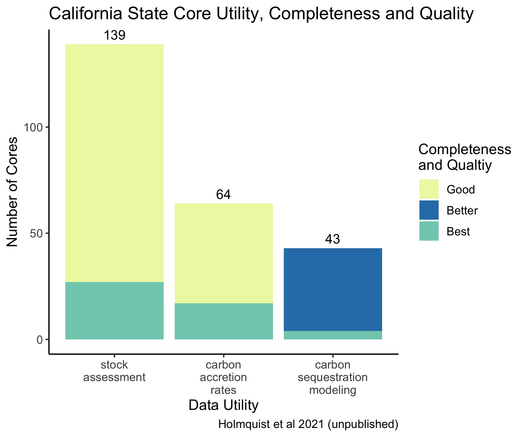
Figure 4.6: California State Core Data Utility, Completeness, and Quality.

Table 4.1: Core counts by utility category, and total, for data sources originating from California.

study_id	stocks	dated cores	elevation measurements	other utility	Total	citation
Callaway et al. 2019	53	41	39	0	53	(John C. Callaway et al. 2019, 2012a)
Watson and Byrne 2013	24	13	0	0	24	(Watson and Byrne 2013)
Kauffman et al. 2020	18	0	0	0	18	(J. Boone Kauffman et al. 2020; Kauffman et al. 2020)
Nahlik and Fennessy 2016	18	0	0	0	18	(Nahlik and Fennessy 2016)
Windham Meyers et al. 2010	16	0	0	0	16	(James R. Holmquist et al. 2018; Windham-Myers et al. 2010)
Weis et al. 2001	6	6	0	0	6	(Daniel A. Weis, Callaway, and Gersberg 2001; Daniel Anthony Weis 1999)
Drexler et al. 2009	3	3	3	0	3	(Drexler, de Fontaine, and Brown 2009)
Buffington et al. 2020	1	1	1	0	1	(Buffington et al. 2020)

4.3.3 Spatial Representativeness

California scores relatively low for spatial coverage due to a spatially clustered sampling effort attributed to the large number of cores taken in the San Francisco Bay area (Figure 4.4C, Figure 4.7). Spatial coverage can be increased by working to distribute the sampling effort more evenly across the state’s wetlands. Lauren Brown of Bowling Green State University (BGSU) is currently processing a data release with the Coastal Carbon Network, which will improve spatial coverage, adding data for several sites along the expanse of the California Coast including Tijuana Estuary, Mission Bay, Newport Bay, Seal Beach, Point Mugu, Morro Bay, Bolinas Lagoon, Bodega Bay, and Humboldt Bay.

Figure 4.7: Spatial distribution of soil cores across California state Blue Carbon habitats.

4.3.4 State Habitat Representation

Based on estimates of aerial coverage, the wetland habitat composition of this state is over 75% tidal marsh. In order of decreasing coverage, the remaining wetland habitat is composed of estuarine aquatic beds (EABs) consisting of seagrasses, algal mats, and kelp, followed by scrub/shrub and swamp. Compared to the sampled representation of these habitats in our database, sampling in California is biased toward tidal marsh and swamp habitats, while EABs are slightly under-represented and the sampling of scrub/shrub is absent. Therefore, habitat representation in this state would benefit from improved sampling coverage of EAB and scrub/shrub habitats. (Figure 4.8, Table 4.2)

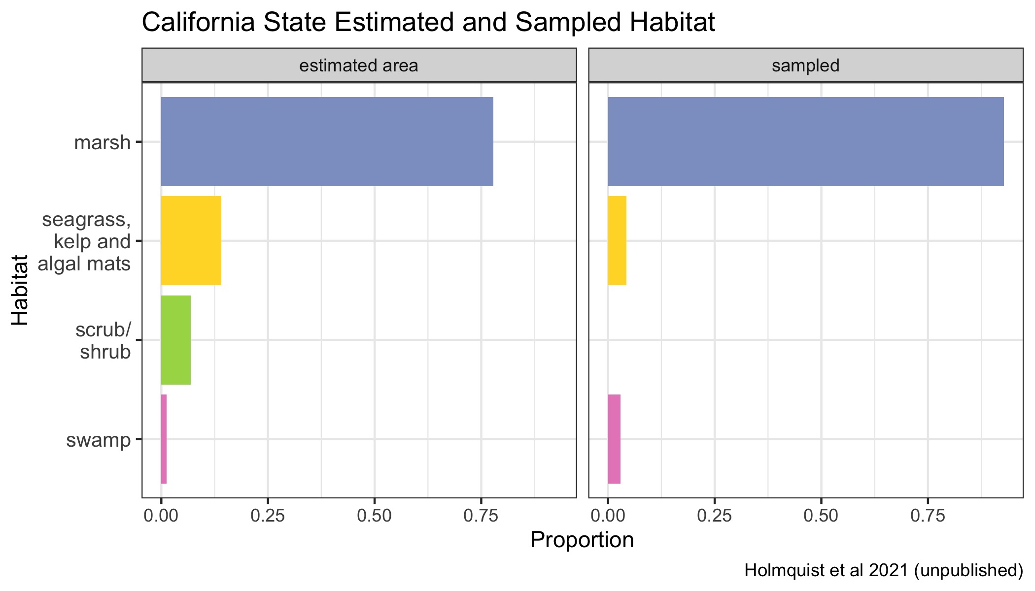
Figure 4.8: Proportions of various Blue Carbon habitats across California state represented in the dataset in proportion to their estimated area. Seagrasses, kelp beds and algal mats are all combined into a single category, because they are combined in the underlying mapping products.

Table 4.2: Estimated areas and carbon stocks assuming 1 m deposit depth, for select natural tidal wetland ecosystem types in California. Estimated areas for potential restoration cases.

Class	Area (Ha)	Million Tonnes C
marsh	45029.5	12.2
seagrass, kelp and algal mats	8118.6	NA
scrub/shrub	4015.0	1.1
swamp	683.4	0.2
total natural	57846.5	13.4

4.3.5 Forthcoming Data

California has 59 forthcoming cores contributed by Lauren Brown of BGSU These data are well distributed along the Californian coast and will improve the spatial coverage for the state, as well as its habitat coverage.

4.4 Florida State Report

4.4.1 State Overview

Florida has 466 cores documented in the Coastal Carbon Atlas or 12.6% of the total number of cores sampled in CONUS. Soil cores from this state score well across metrics of quality, spatial and habitat coverage, but fall short of the median in terms of quantity. Despite having a large percentage of documented cores in the Atlas, Florida scores the lowest in representative quantity because of the disproportionately large amount of wetland habitat found in this state (21.8% of the total wetland area in CONUS) (Figure 4.10, Figure 4.9A). This highlights a general need for increased sampling effort in this state.

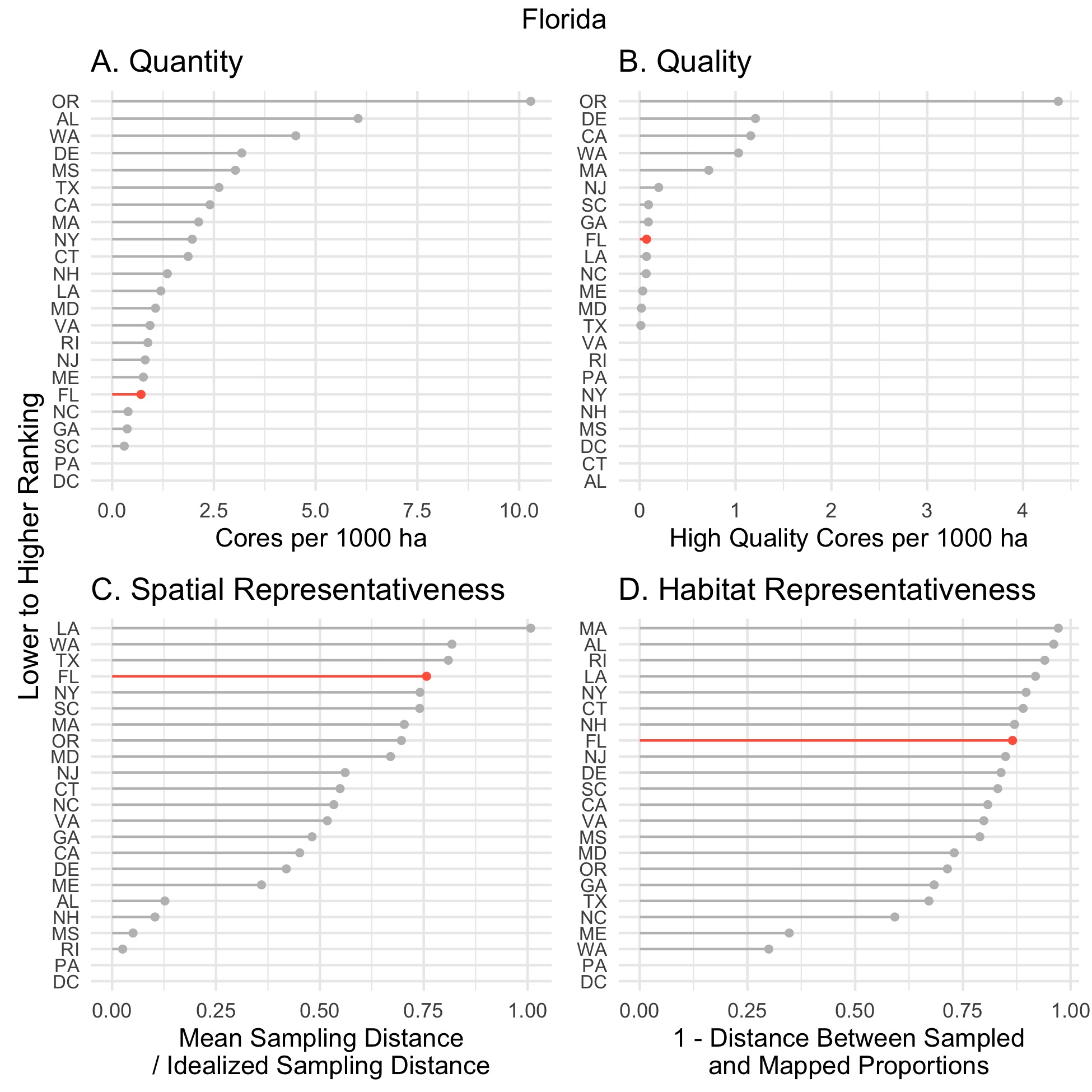
Figure 4.9: State ranking on all four soil Blue Carbon metrics, A. Quantity, B. Quality, C. Spatial Representativeness, D. Habitat Representativeness.

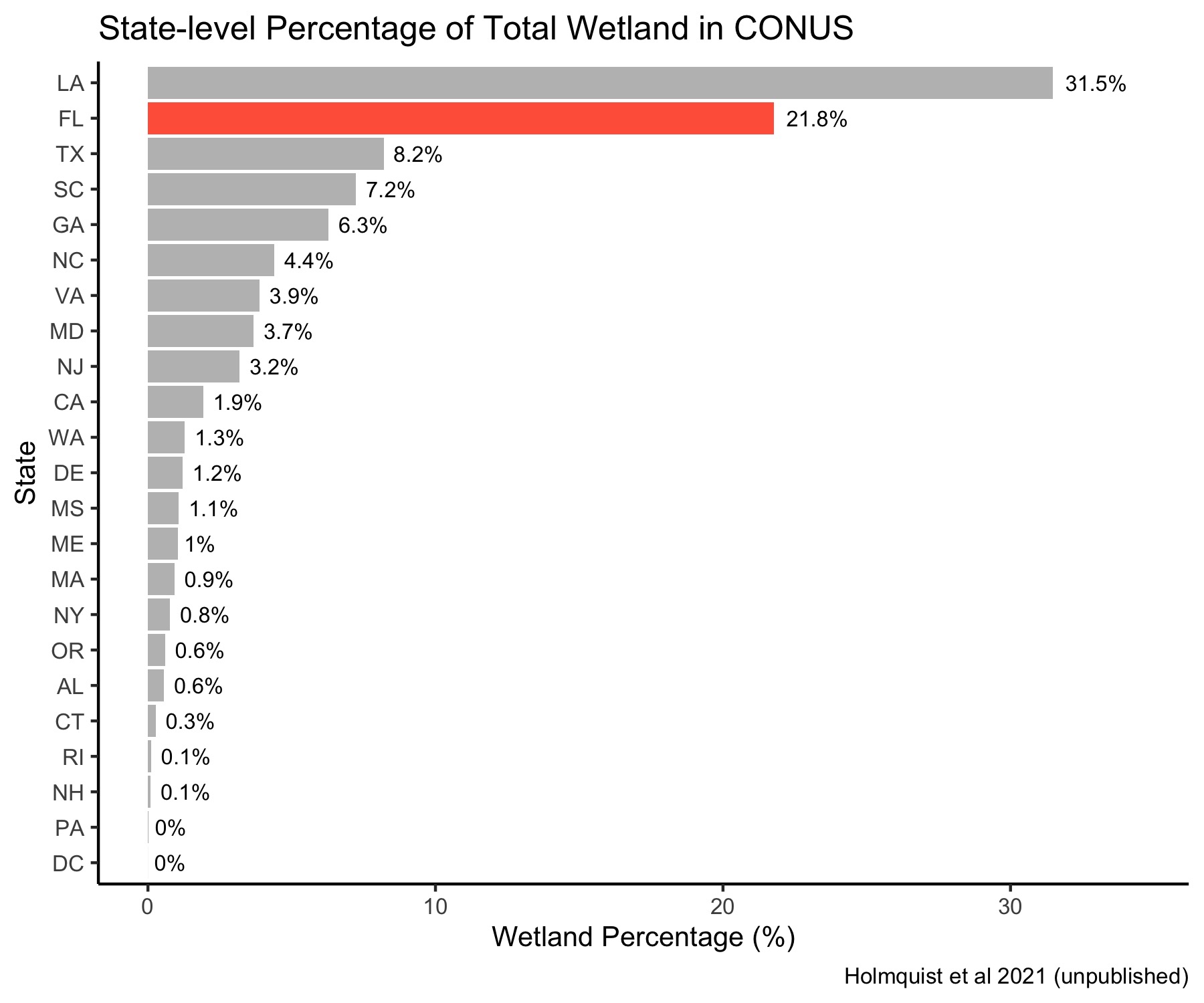
Figure 4.10: State-Level Wetland Contribution

4.4.2 Data Utility and Availability

The quality of the soil core data from Florida is relatively fair but would benefit from increased representation of soil cores with dating information and precise elevation (Figure 4.9B). While the majority of cores can be used for carbon stock assessments, less than 10% can be used for carbon accretion rate assessments and almost no cores in Florida can be used for carbon sequestration modeling because the cores lack precise elevation data. Fortunately, the dated cores that are available for Florida have detailed information and many cores confirmed to reach the bottom of the deposit; peat deposits along the Everglades tend to be very thin, making this an easier bar to clear compared to wetlands with deeper deposits. (Figure 4.11, Table 4.3)

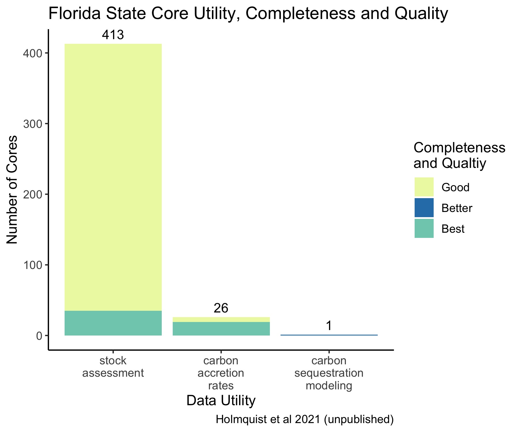
Figure 4.11: Florida State Core Data Utility, Completeness, and Quality.

Table 4.3: Core counts by utility category, and total, for data sources originating from Florida

study_id	stocks	dated cores	elevation measurements	other utility	Total	citation
Osland et al. 2016	193	0	0	0	193	(Osland et al. 2016)
Doughty et al. 2016	68	0	0	0	68	(C. Doughty et al. 2019; C. L. Doughty et al. 2016)
Nahlik and Fennessy 2016	34	0	0	0	34	(Nahlik and Fennessy 2016)
Lewis et al. 2007	0	0	0	26	26	(Fourqurean et al. 2012; Lewis et al. 2007)
Fourqurean et al. 2010	24	0	0	0	24	(Fourqurean et al. 2012; Fourqurean, Muth, and Boyer 2010)
Breithaupt et al. 2017	20	0	0	0	20	(James R. Holmquist et al. 2018; Joshua L. Breithaupt et al. 2017)
Grady 1981	0	0	0	10	10	(Fourqurean et al. 2012; Grady 1981)
Osland et al. 2012	9	0	0	0	9	(Sanderman 2017; Osland et al. 2012)
Fourqurean unpublished	8	0	0	0	8	(Fourqurean et al. 2012)
Orem et al. 1999	0	0	0	8	8	(Fourqurean et al. 2012; Orem et al. 1999)
Breithaupt et al. 2020	7	7	0	0	7	(Breithaupt et al. 2020)
Marchio et al. 2016	7	0	0	0	7	(Sanderman 2017; Marchio et al. 2016)
NCSS	7	0	0	0	7	[NA]
Arriola and Cable 2017	6	6	0	0	6	(Arriola and Cable 2017)
Breithaupt et al. 2014	6	6	0	0	6	(Joshua L. Breithaupt et al. 2014; Joshua L. Breithaupt et al. 2019)
Vaughn et al. 2020	6	6	0	0	6	(D. Vaughn et al. 2020)
Radabaugh et al. 2018	5	0	0	0	5	(James R. Holmquist et al. 2018; Radabaugh et al. 2018)
Yarbro and Carlson 2008	0	0	0	5	5	(Fourqurean et al. 2012; Yarbro and Carlson Jr 2008)
Cahoon and Lynch 1997	4	0	0	0	4	(Sanderman 2017; Cahoon et al. 1997)
Chen and Twilley 1999	4	0	0	0	4	(Sanderman 2017; Chen and Twilley 1999)
Chmura et al. 2003	0	0	0	2	2	(Sanderman 2017; Chmura et al. 2003)
Gerlach et al. 2017	2	1	1	0	2	(Gerlach et al. 2017)
Burns and Swart 1992	0	0	0	1	1	(Fourqurean et al. 2012; BURNS and SWART 1992)
Callaway et al. 1997	1	0	0	0	1	(Sanderman 2017; Callaway et al. 1997)
Rosenfeld 1979	0	0	0	1	1	(Fourqurean et al. 2012; Rosenfeld 1979)
Smoak et al. 2013	1	0	0	0	1	(Sanderman 2017; Smoak et al. 2013)
Yando et al. 2016	1	0	0	0	1	(Sanderman 2017; Yando et al. 2016)

4.4.3 Spatial Representativeness

Soil core sampling efforts in Florida are sparsely, yet evenly distributed across the state’s watersheds, resulting in high spatial coverage (Figure 4.9C, Figure 4.12).

Figure 4.12: Spatial distribution of soil cores across Florida state Blue Carbon habitats.

4.4.4 State Habitat Representation

Florida presents the most diverse assortment of Blue Carbon habitats sampled. In order of decreasing coverage, the aerial estimates of tidal wetlands include marsh, mangrove, EAB (seagrass, kelp and algal mats), scrub/shrub, and swamp habitats. There is a slight bias toward mangrove and EAB habitats while marsh and scrub/shrub habitats are underrepresented. Overall, the estimated area of habitat types are fairly represented in sampling coverage, but there is room for improvement. (Figure 4.13, Table 4.4)

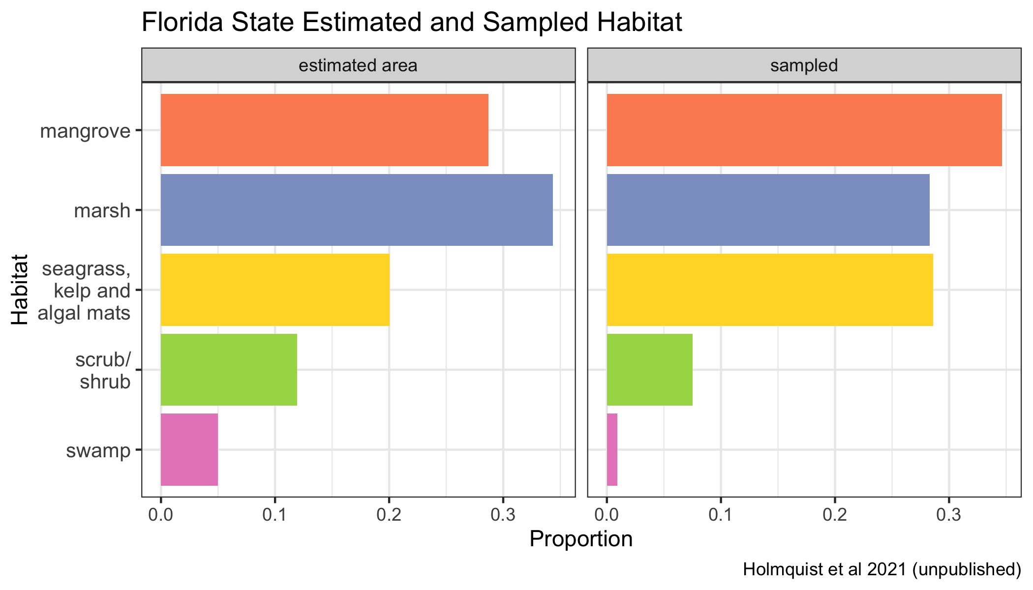
Figure 4.13: Proportions of various Blue Carbon habitats across Florida state represented in the dataset in proportion to their estimated area. Seagrasses, kelp beds and algal mats are all combined into a single category, because they are combined in the underlying mapping products.

Table 4.4: Estimated areas and carbon stocks assuming 1 m deposit depth, for select natural tidal wetland ecosystem types in Florida. Estimated areas for potential restoration cases.

Class	Area (Ha)	Million Tonnes C
marsh	225610.9	60.9
mangrove	188386.1	50.9
seagrass, kelp and algal mats	131484.8	NA
scrub/shrub	78197.4	21.1
swamp	32734.0	8.8
total natural	656413.1	141.7

4.4.5 Forthcoming Data

Florida has over 100 forthcoming cores in prep for data release by the Coastal Carbon Network. These cores are contributed by Dr. André Rovai of Louisiana State University, Dr. Lisa Schile-Beers of Silvestrum Climate Associates and the Smithsonian Environmental Research Center (SERC), and Claire Fell and Dr. Samantha Chapman of Villanova University. These additional data will increase the coverage and quantity of cores per total wetland area of Florida, the latter of which is an area that is currently under-represented for the state.

4.5 Maine State Report

4.5.1 State Overview

Maine is represented in the Coastal Carbon Atlas by 24 cores, which amounts to less than 1% of the total number of cores available for CONUS. This state scores at or below the median across all Blue Carbon metrics (Figure 4.14), highlighting a need for more data to be made available for this state or more targeted sampling efforts to be made which collectively increase the quantity, quality, and coverage of it’s inventory.

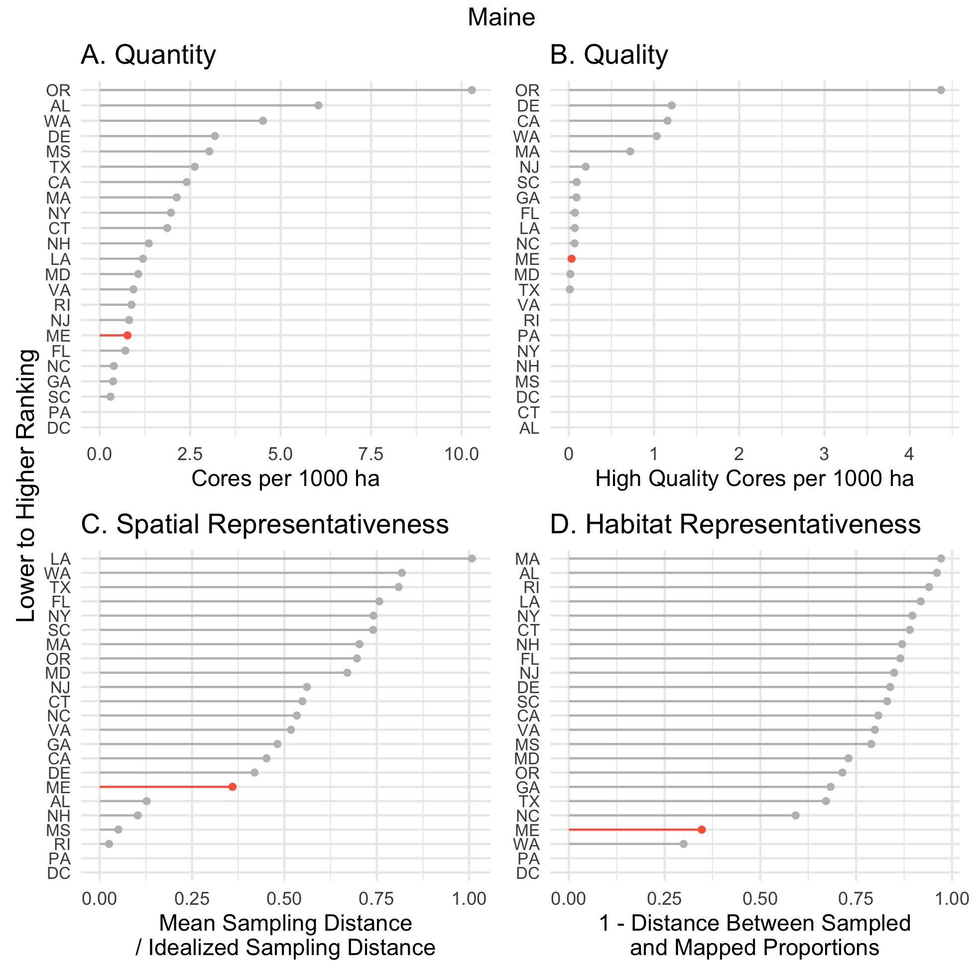
Figure 4.14: State ranking on all four soil Blue Carbon metrics, A. Quantity, B. Quality, C. Spatial Representativeness, D. Habitat Representativeness.

Figure 4.15: State-Level Wetland Contribution

4.5.2 Data Utility and Availability

The quality of the soil core data from Maine is poor compared with other states (Figure 4.14B). All 24 documented cores can be used for carbon stock assessments, however, only one contains viable information for carbon accretion rate assessments. (Figure 4.16, Table 4.5)

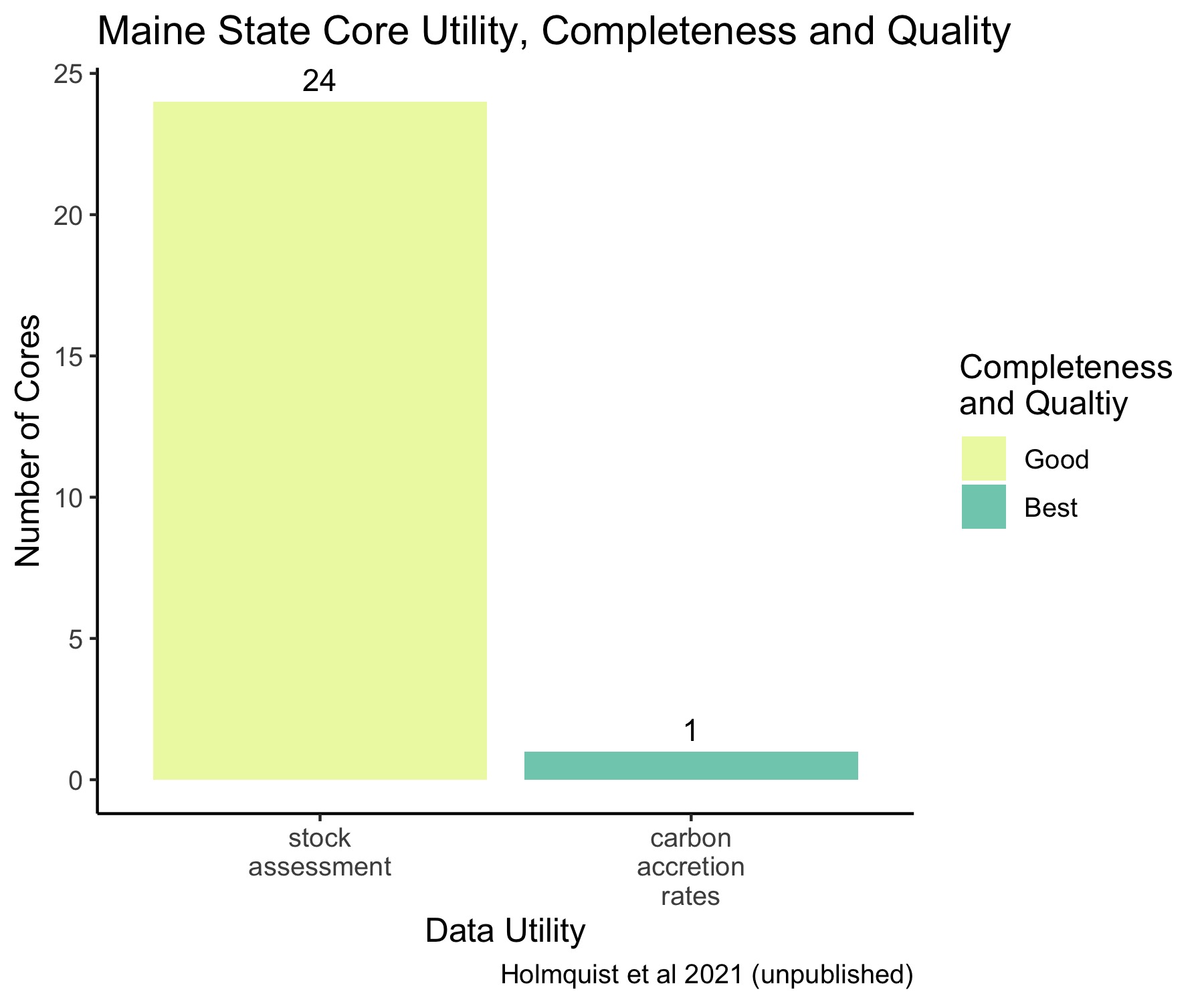
Figure 4.16: Maine State Core Data Utility, Completeness, and Quality.

Table 4.5: Core counts by utility category, and total, for data sources originating from Maine

study_id	stocks	dated cores	elevation measurements	other utility	Total	citation
Drake et al. 2015	20	0	0	0	20	(James R. Holmquist et al. 2018; Drake et al. 2015)
Nahlik and Fennessy 2016	3	0	0	0	3	(Nahlik and Fennessy 2016)
Johnson et al. 2007	1	1	0	0	1	(Johnson et al. 2007)

4.5.3 Spatial Representativeness

Maine is poorly represented at a spatial scale, largely due to the low quantity of cores available through the Atlas. Additionally, the majority of soil cores from this state were contributed through one study which sampled along the lower half of the coastline (Drake et al. 2015). Subsequently, this state’s spatial representativeness score could be improved through increased sampling of coastal wetlands in the mid to higher latitudes of the state. (Figure 4.14C, Figure 4.17)

Figure 4.17: Spatial distribution of soil cores across Maine state Blue Carbon habitats.

4.5.4 State Habitat Representation

Maine contributes a small percentage of the total CONUS coastal wetland, however, it contains a rich assortment of Blue Carbon habitats. This state ranks low in habitat representativeness because only marsh habitats have been sampled in this state, which is estimated to contain notable amounts of swamp and estuarine aquatic bed (seagrass, kelp and algal mats) habitats. Habitat coverage in this state can be improved through increased sampling of these underrepresented habitats. (Figure 4.18, Table 4.6)

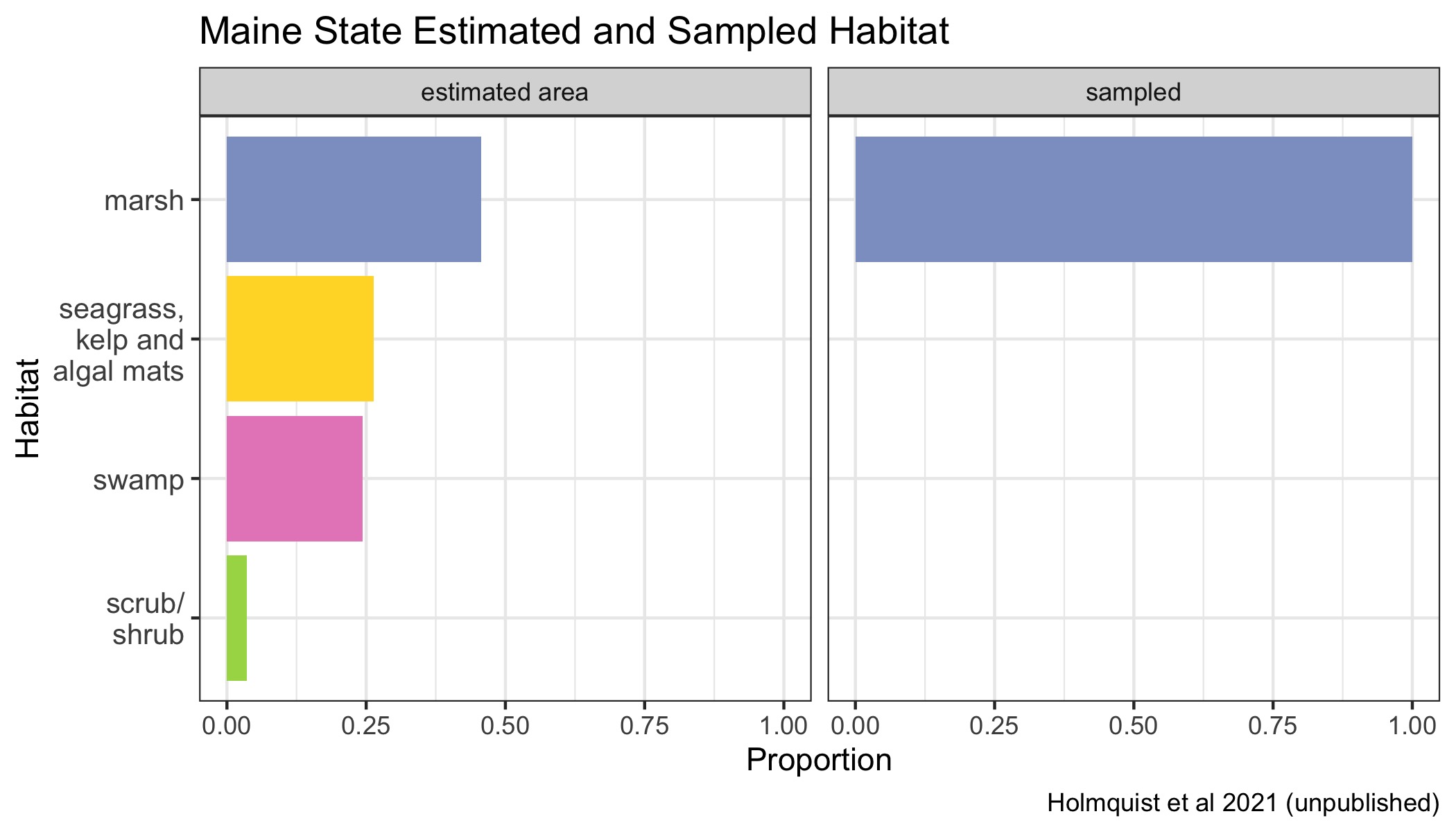
Figure 4.18: Proportions of various Blue Carbon habitats across Maine represented in the dataset in proportion to their estimated area. Seagrasses, kelp beds and algal mats are all combined into a single category, because they are combined in the underlying mapping products.

Table 4.6: Estimated areas and carbon stocks assuming 1 m deposit depth, for select natural tidal wetland ecosystem types in Maine. Estimated areas for potential restoration cases.

Class	Area (Ha)	Million Tonnes C
marsh	14270.2	3.9
seagrass, kelp and algal mats	8244.8	NA
swamp	7642.2	2.1
scrub/shrub	1135.4	0.3
total natural	31292.6	6.2

4.5.5 Forthcoming Data

There are currently 45 soil cores in prep for data release by the Coastal Carbon Network, contributed by Dr. Beverly Johnson of Bates College. Once these data are made publicly available, they will almost triple the current inventory of soil cores for Maine and will greatly increase the spatial sampling coverage.

4.6 Maryland State Report

4.6.1 State Overview

Maryland contains 118 cores, which represents 3.2% of the total number of cores sampled in CONUS. This state’s score lies near the median across all Blue Carbon metrics relative to other coastal CONUS states (Figure 4.19). Given that this state contains 3.7% of the total wetland acreage in CONUS, more soil cores will be needed to increase its representative quantity score (Figure 4.20). This presents room for inventory improvement, particularly through more sampling in habitat types other than marshes and increasing the availability of high-quality soil core data.

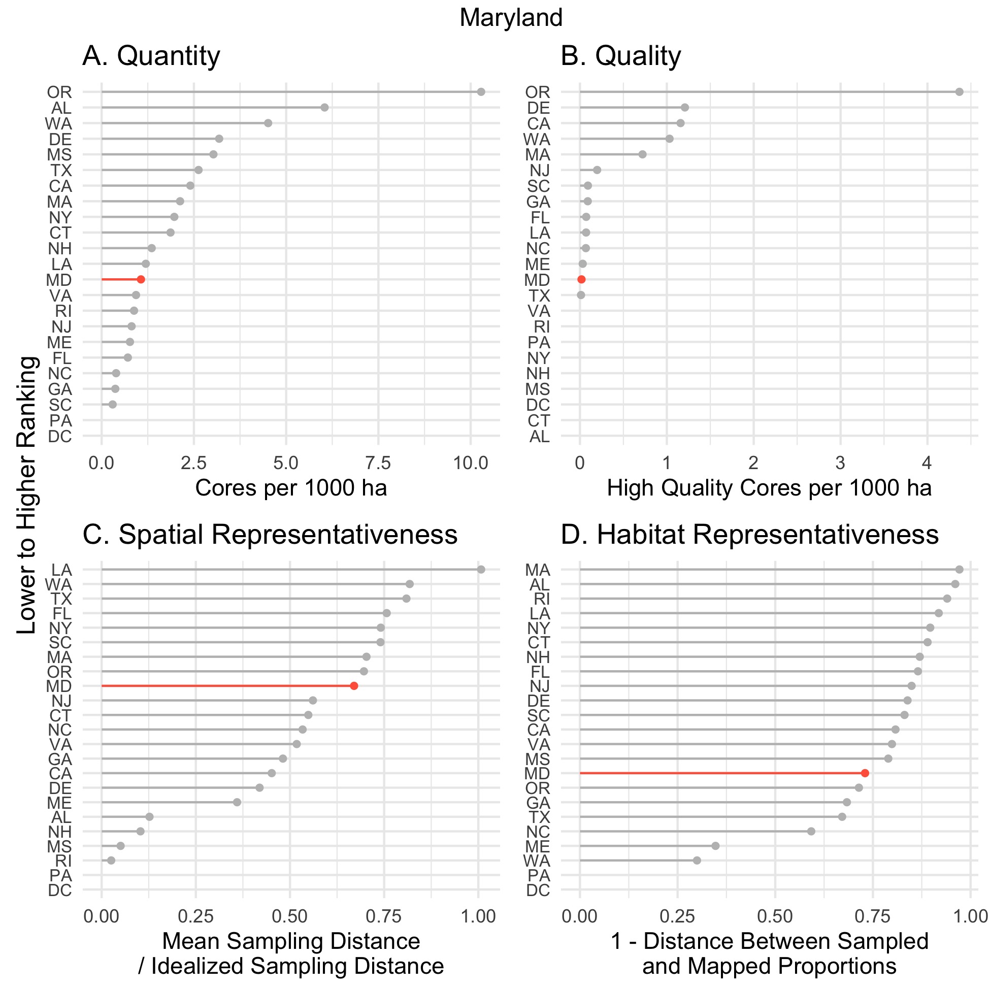
Figure 4.19: State ranking on all four soil Blue Carbon metrics, A. Quantity, B. Quality, C. Spatial Representativeness, D. Habitat Representativeness.

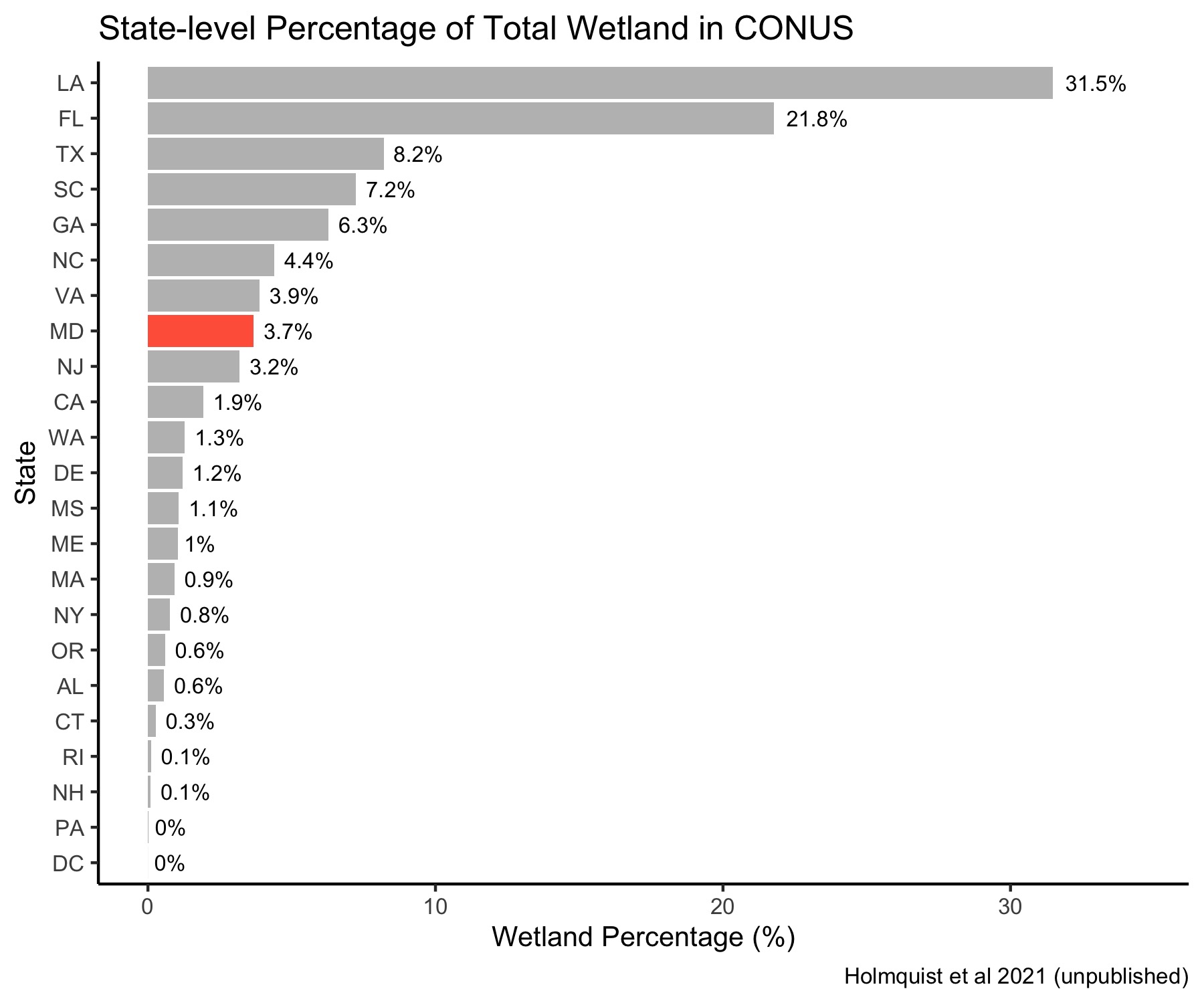
Figure 4.20: State-Level Wetland Contribution

4.6.2 Data Utility and Availability

The quality of the soil core data from Maryland is fair relative to other Pew-selected states (Figure 4.19B). While almost all cores can be used for carbon stock assessments, less than 10% can be used for carbon accretion rate assessments, and almost no cores can be used for carbon sequestration modeling because the cores lack precise elevation data (Figure 4.21, Table 4.7). Adding more soil cores to this state’s inventory with dating and elevation information would increase it’s utility and enable it’s application to a wider variety of Blue Carbon projects.

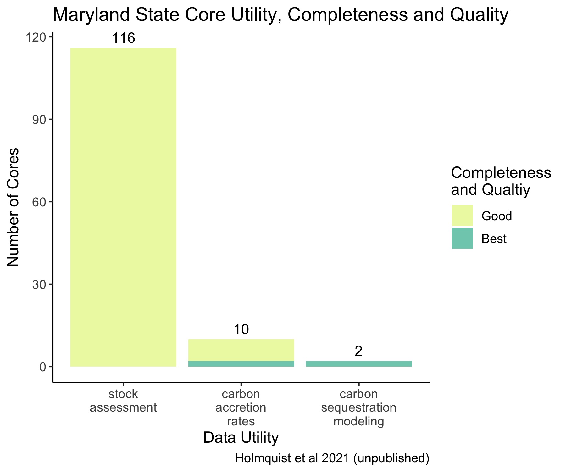
Figure 4.21: Maryland State Core Data Utility, Completeness, and Quality.

Table 4.7: Core counts by utility category, and total, for data sources originating from Maryland

study_id	stocks	dated cores	elevation measurements	other utility	Total	citation
Merrill 1999	37	0	0	0	37	(James R. Holmquist et al. 2018; Merrill 1999)
Nahlik and Fennessy 2016	22	0	0	2	24	(Nahlik and Fennessy 2016)
Keshta et al. 2020 a	21	0	0	0	21	(El Shahat Sedik Keshta, Yarwood, and Baldwin 2020; El Shahat Sedik Keshta 2017)
Pastore et al. 2017	20	0	0	0	20	(James R. Holmquist et al. 2018; Pastore, Megonigal, and Langley 2017)
Ensign et al. 2020	8	8	0	0	8	(Ensign et al. 2015)
Keshta et al. 2020 b	6	0	0	0	6	(El Shahat Sedik Keshta, Yarwood, and Baldwin 2020; El Shahat Sedik Keshta 2017)
Messerschmidt and Kirwan 2020	2	2	2	0	2	(Messerschmidt and Kirwan 2020)

4.6.3 Spatial Representativeness

Maryland fell near the median among Pew-selected states for spatial representativeness, which indicates a fairly evenly distributed sampling effort across the state (Figure 4.19C, Figure 4.22). This could be improved through increased sampling of coastal wetlands at the north and south of the Chesapeake Bay.

Figure 4.22: Spatial distribution of soil cores across Maryland state Blue Carbon habitats.

4.6.4 State Habitat Representation

The composition of Blue Carbon habitats in this state are 75% marsh, followed by swamp, scrub/shrub, and a small amount of EAB. There is a bias toward marshes, while swamps are underrepresented, and sampling of scrub/shrub and EAB habitats is absent. Maryland’s habitat coverage score could be improved through more sampling of swamp, scrub/shrub, and EAB. (Figure 4.23, Table 4.8)

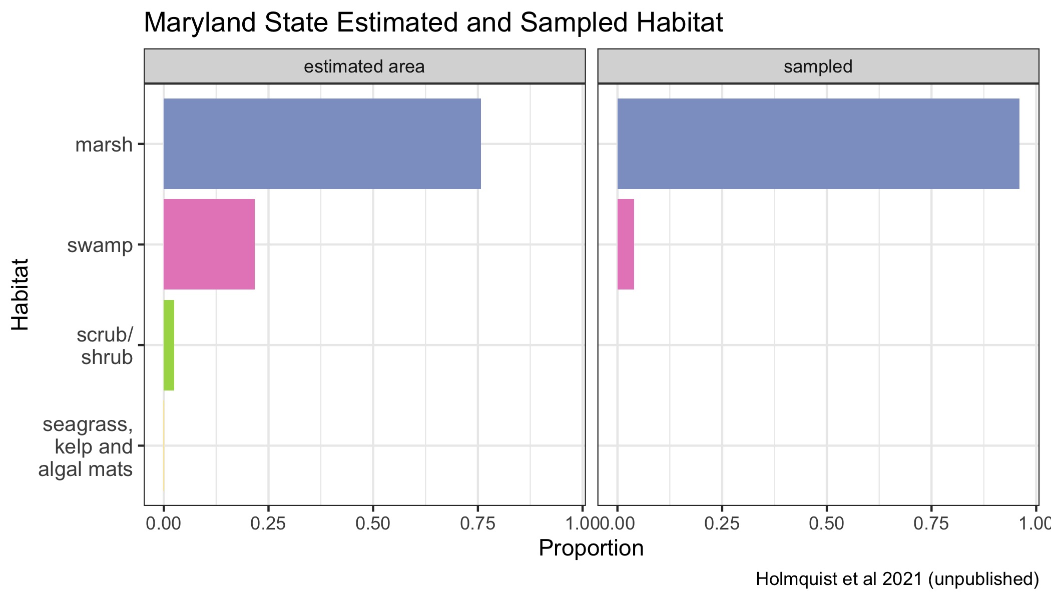
Figure 4.23: Proportions of various Blue Carbon habitats across Maryland state represented in the dataset in proportion to their estimated area. Seagrasses, kelp beds and algal mats are all combined into a single category, because they are combined in the underlying mapping products.

Table 4.8: Estimated areas and carbon stocks assuming 1 m deposit depth, for select natural tidal wetland ecosystem types in Maryland. Estimated areas for potential restoration cases.

Class	Area (Ha)	Million Tonnes C
marsh	83928.8	22.7
swamp	24054.9	6.5
scrub/shrub	2763.6	0.7
seagrass, kelp and algal mats	34.1	NA
total natural	110781.4	29.9

4.6.5 Forthcoming Data

Maryland has 20 forthcoming cores from Dr. Patrick Megonigal of SERC that will increase the state’s core count and subsequently its representative quantity score. Dr. Timothy Shaw of the Earth Observatory of Singapore is contributing a forthcoming core from the Global Change Research Wetland that will be level A1, highest quality. Many cores from Merrill (1999) have lead-210 dating information, however this data is recorded in a print dissertation and needs to be digitized. We are also aware of many other unpublished soil core datasets, and are continuing to reach out and offer assistance to researchers in the regions.

4.7 Massachusetts State Report

4.7.1 State Overview

Massachusetts has 59 cores or 1.6% of the total number of tidal wetland cores in the Atlas for CONUS. Massachusetts had the highest composite rank, scoring well across all four categories. The state contains many high quality cores relative to its wetland area which we attribute to the high volume of relevant research being conducted in the this region. Relative to other coastal states, the quantity of soil cores sampled in this state is fairly representative but could be improved (Figure 4.24A). Massachusetts’ overall score can continue to improve through the collection of more high-quality cores.

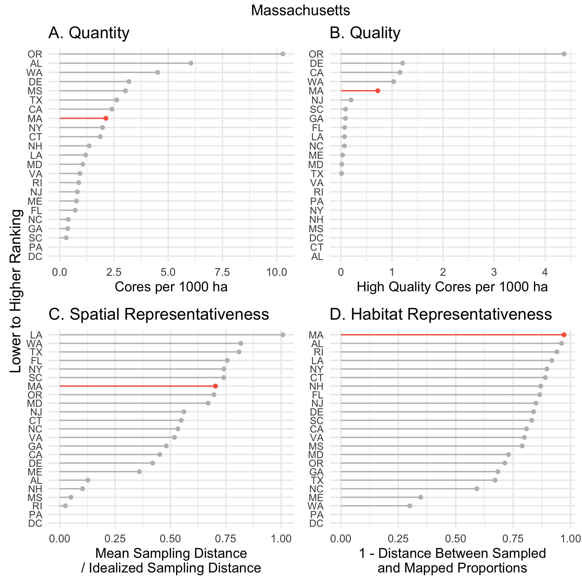
Figure 4.24: State ranking on all four soil Blue Carbon metrics, A. Quantity, B. Quality, C. Spatial Representativeness, D. Habitat Representativeness.

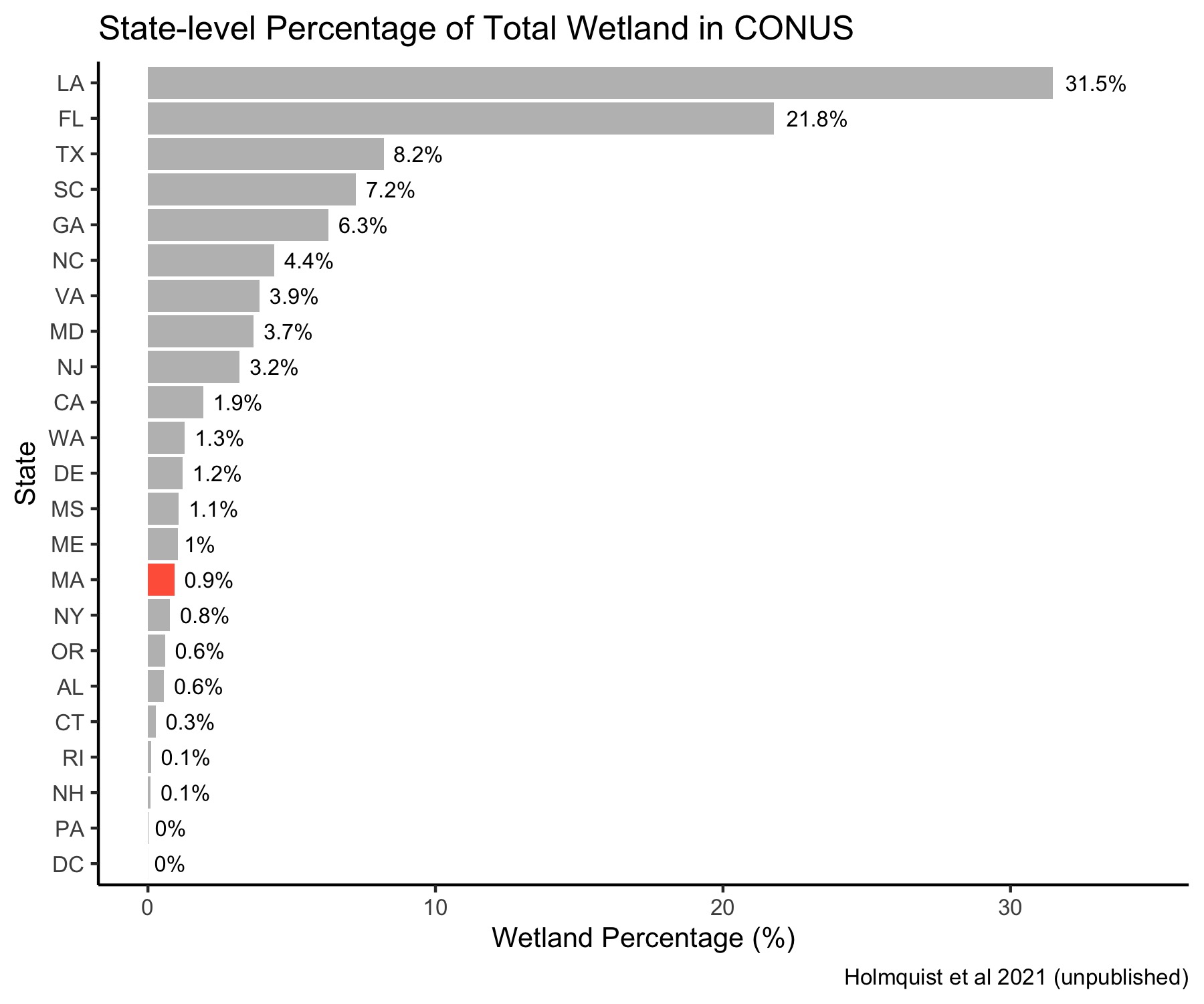
Figure 4.25: State-Level Wetland Contribution

4.7.2 Data Utility and Availability

The quality of the soil core data from Massachusetts is considerably high relative to other states (Figure 4.24B). Of the cores which can be used for carbon stock assessments, about half are viable for carbon accretion rate assessments, and over a third of the cores can be used for carbon sequestration modeling. (Figure 4.26, Table 4.9)

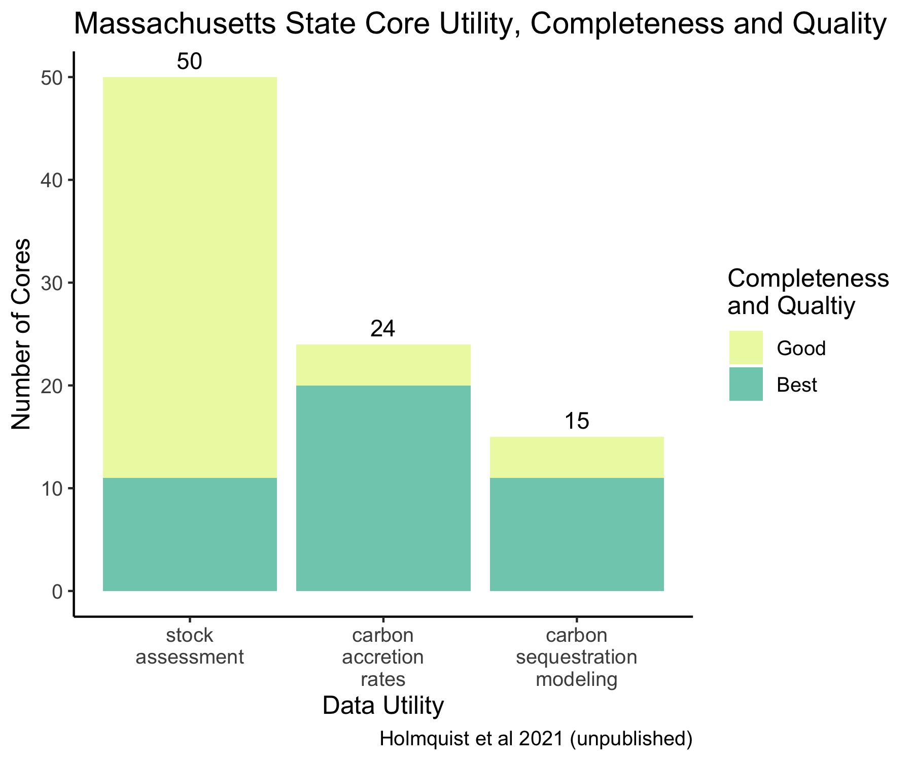
Figure 4.26: Massachusetts State Core Data Utility, Completeness, and Quality.

Table 4.9: Core counts by utility category, and total, for data sources originating from Massachusetts

study_id	stocks	dated cores	elevation measurements	other utility	Total	citation
Drake et al. 2015	20	0	0	0	20	(James R. Holmquist et al. 2018; Drake et al. 2015)
Gonneea et al. 2018	11	11	11	0	11	(Gonneea, Kroeger, and O’Keefe-Suttles 2018)
Luk et al. 2020 a	9	0	0	0	9	(Sheron Y. Luk et al. 2021; Amanda Spivak 2020)
Luk et al. 2020 b	0	9	0	0	9	(Sheron Y. Luk et al. 2021; Sheron Y. Luk et al. 2020)
Nahlik and Fennessy 2016	6	0	0	0	6	(Nahlik and Fennessy 2016)
Giblin and Forbrich 2018	4	4	4	0	4	(Giblin, Forbrich, and Plum Island Ecosystems LTER 2018)

4.7.3 Spatial Representativeness

Relative to other coastal states, Massachusetts scores very high for spatial coverage (Figure 4.24C, Figure 4.27). This is indicative of the evenly distributed sampling effort across the state. Two research hotspots of note are the Plum Island Ecosystems Long-Term Ecological Research (LTER) Site and USGS Woods Hole’s site at Waquoit Bay National Estuarian Research Reserve. The sites are spread out across the north and south side of the states’ coast, respectively, helping it score well on spatial representativeness.

Figure 4.27: Spatial distribution of soil cores across Massachusetts state Blue Carbon habitats.

4.7.4 State Habitat Representation

Based on mapped estimates of habitat type, Massachusetts wetland composition is over 90% marsh, with small amounts of swamp, scrub/shrub, and estuarine aquatic bed (EAB; seagrass, kelp bed and algal map) habitat. Compared to other states, Massachusetts scores well for habitat coverage. The soil core sampling in this state is representative of these habitats. There is an absence of samples from scrub/shrub and EAB habitat, but the impact is offset because the proportional area of these habitats is small. (Figure 4.28, Table 4.10)

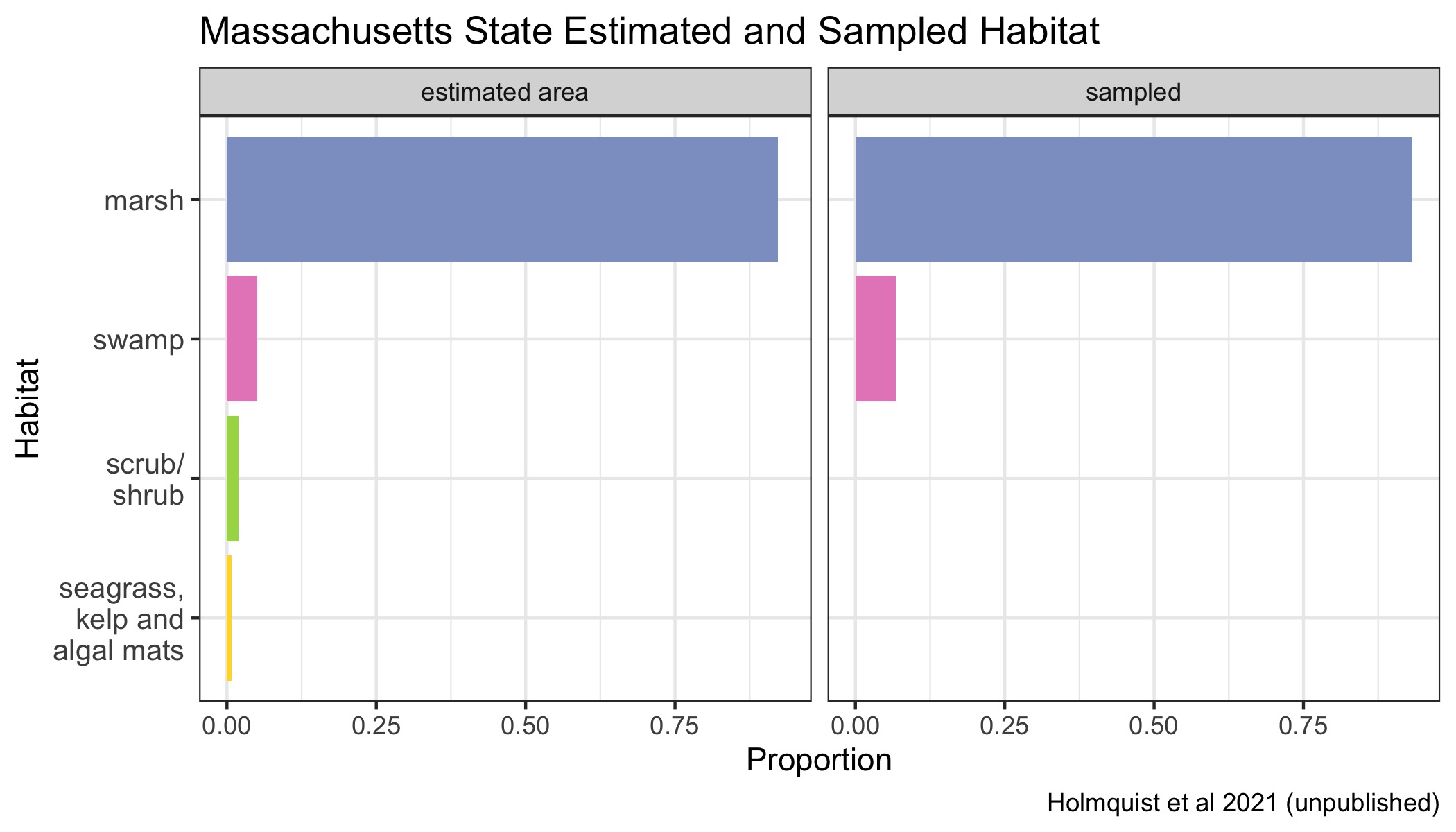
Figure 4.28: Proportions of various Blue Carbon habitats across Massachusetts state represented in the dataset in proportion to their estimated area. Seagrasses, kelp beds and algal mats are all combined into a single category, because they are combined in the underlying mapping products.

Table 4.10: Estimated areas and carbon stocks assuming 1 m deposit depth, for select natural tidal wetland ecosystem types in Massachusetts. Estimated areas for potential restoration cases.

Class	Area (Ha)	Million Tonnes C
marsh	25595.8	6.9
swamp	1413.5	0.4
scrub/shrub	524.0	0.1
seagrass, kelp and algal mats	228.9	NA
total natural	27762.1	7.4

4.7.5 Forthcoming Cores

Dr. Nathaniel Weston of Villanova University is contributing 3 more cores for the Plum Island Ecosystems LTER which are currently in prep for data release by the Coastal Carbon Network. These cores will be viable for carbon stock assessments, carbon accretion rate estimates, and carbon sequestration modeling.

4.8 New Jersey State Report

4.8.1 State Overview

New Jersey contains 78 cores or 2.1% of the total number of cores sampled in CONUS. Overall, this state’s composite score lies slightly above the median, scoring highest on data quality and lowest on representative quantity (Figure 4.29). This state scores below the median on the quantity metric because the number of soil cores sampled in this state does not sufficiently represent the area of coastal wetland estimated for this state. New Jersey’s score can be improved through more soil sampling strategically aimed at increasing spatial coverage in Delaware Bay.

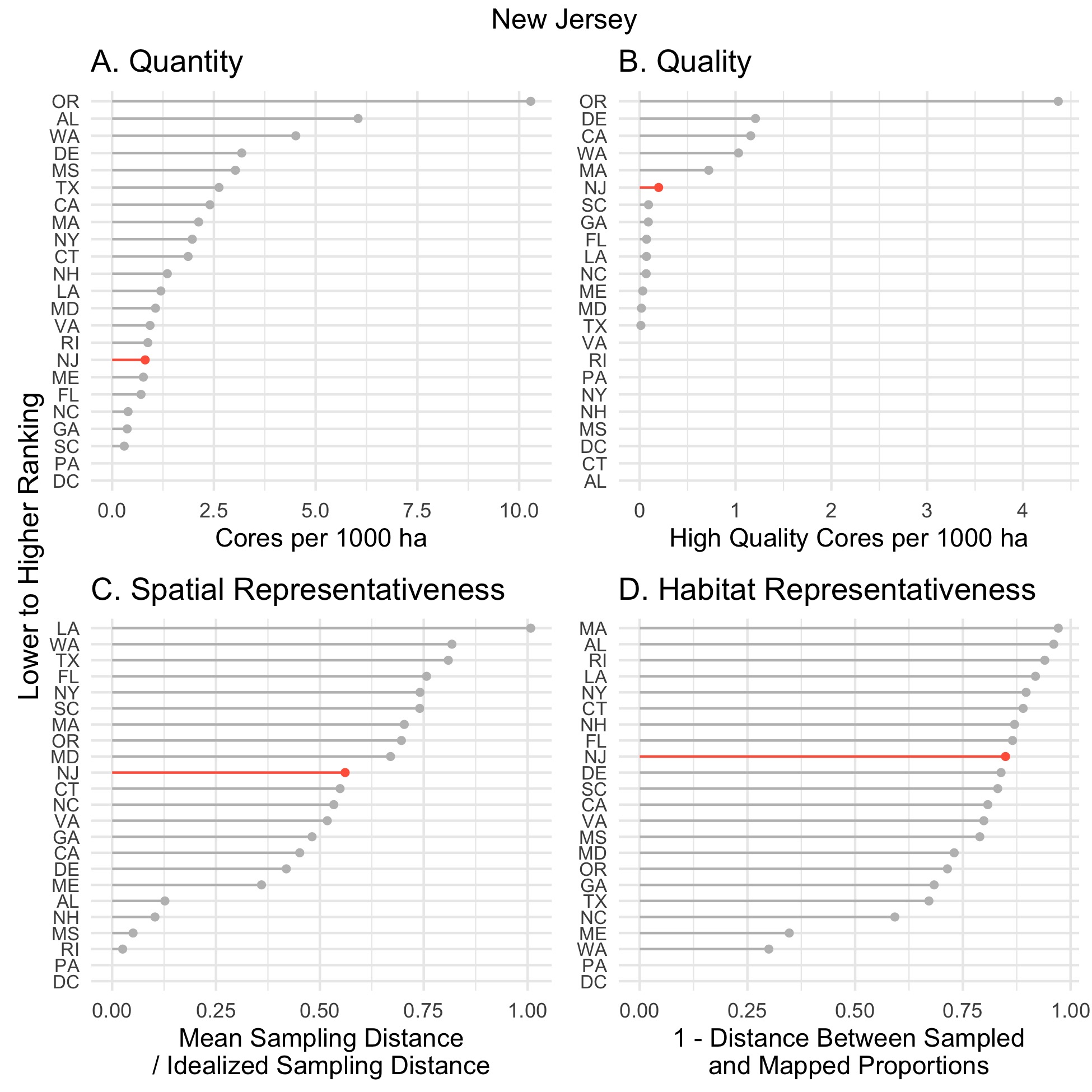
Figure 4.29: State ranking on all four soil Blue Carbon metrics, A. Quantity, B. Quality, C. Spatial Representativeness, D. Habitat Representativeness.

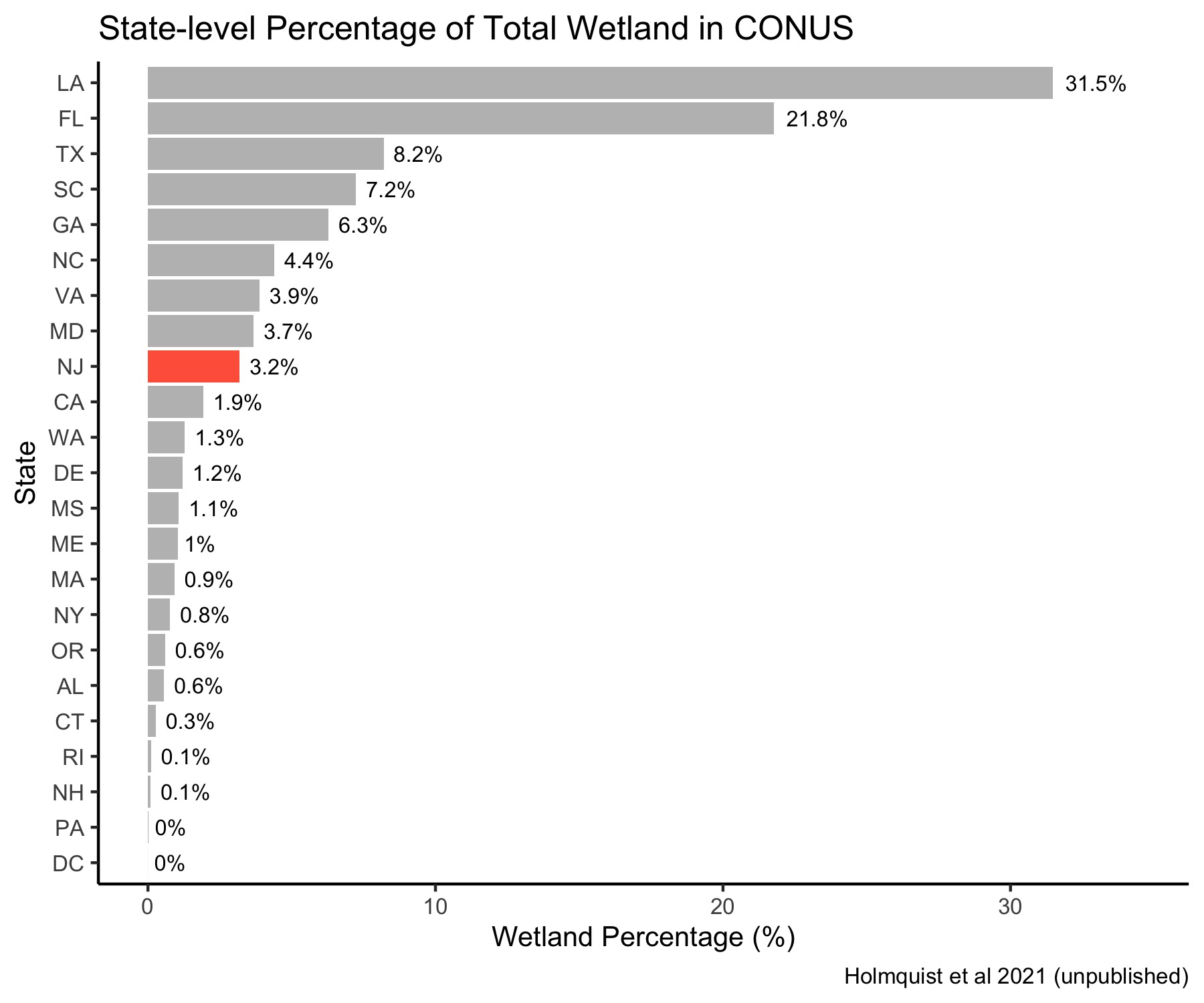
Figure 4.30: State-Level Wetland Contribution

4.8.2 Data Utility and Availability

The quality of the soil core data from New Jersey is good and near the median of Pew-selected Atlantic coast states (Figure 4.29B). All NJ cores present in the Atlas can be used for carbon stock assessments and roughly 25% can be used for carbon accretion rate assessments or carbon sequestration modeling (Figure 4.31, Table 4.11).

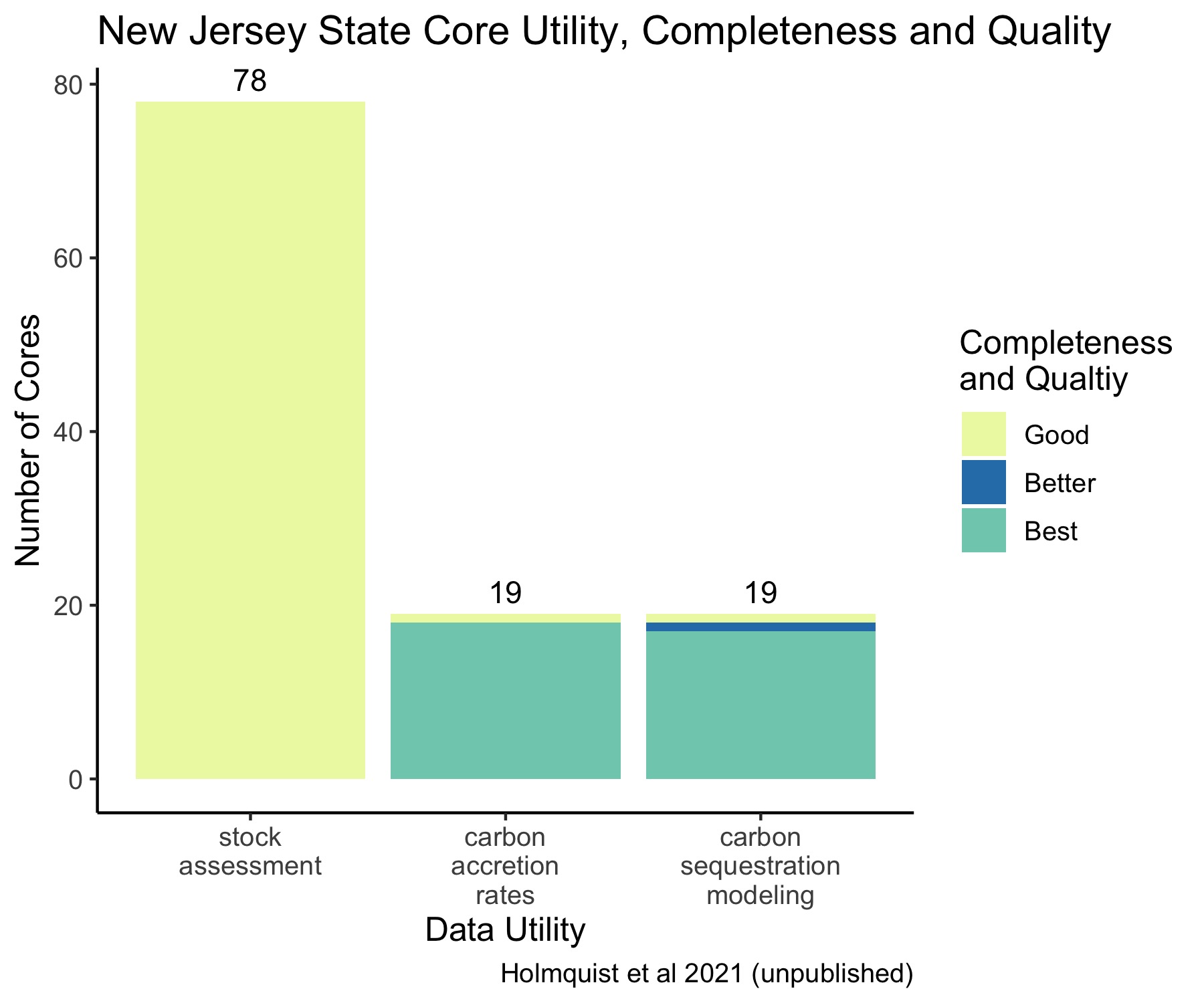
Figure 4.31: New Jersey State Core Data Utility, Completeness, and Quality.

Table 4.11: Core counts by utility category, and total, for data sources originating from New Jersey

study_id	stocks	dated cores	elevation measurements	other utility	Total	citation
Drake et al. 2015	20	0	0	0	20	(James R. Holmquist et al. 2018; Drake et al. 2015)
Boyd et al. 2017	18	18	18	0	18	(B. M. Boyd, Sommerfield, and Elsey-Quirk 2017; B. Boyd et al. 2019)
Unger et al. 2016	18	0	0	0	18	(Unger et al. 2016; B. Boyd et al. 2019)
Nahlik and Fennessy 2016	17	0	0	0	17	(Nahlik and Fennessy 2016)
Orson 1990	4	0	0	0	4	(James R. Holmquist et al. 2018; Richard A. Orson 1990)
Kemp et al. 2020	1	1	1	0	1	(Kemp et al. 2012, 2020)

4.8.3 Spatial Representativeness

Spatial representativeness of Blue Carbon soil data in New Jersey is fair compared to other states, likely due to lack of sampling of the wetlands in the New Jersey portion of Delaware Bay (Figure 4.29C, Figure 4.32).

Figure 4.32: Spatial distribution of soil cores across New Jersey state Blue Carbon habitats.

4.8.4 State Habitat Representation

The coastal wetland composition of New Jersey is an estimated 80% marsh, followed by swamp, scrub/shrub, and a small amount of estuarine aquatic bed (EAB; seagrass, kelp bed and algal mat). There is a sampling bias toward marsh habitat when compared to other Blue Carbon habitat types in New Jersey as it is the only habitat type in the database for this state. Subsequently, this state’s habitat coverage score could be improved through more sampling of swamp, scrub/shrub, and EAB. (Figure 4.33, Table 4.12)

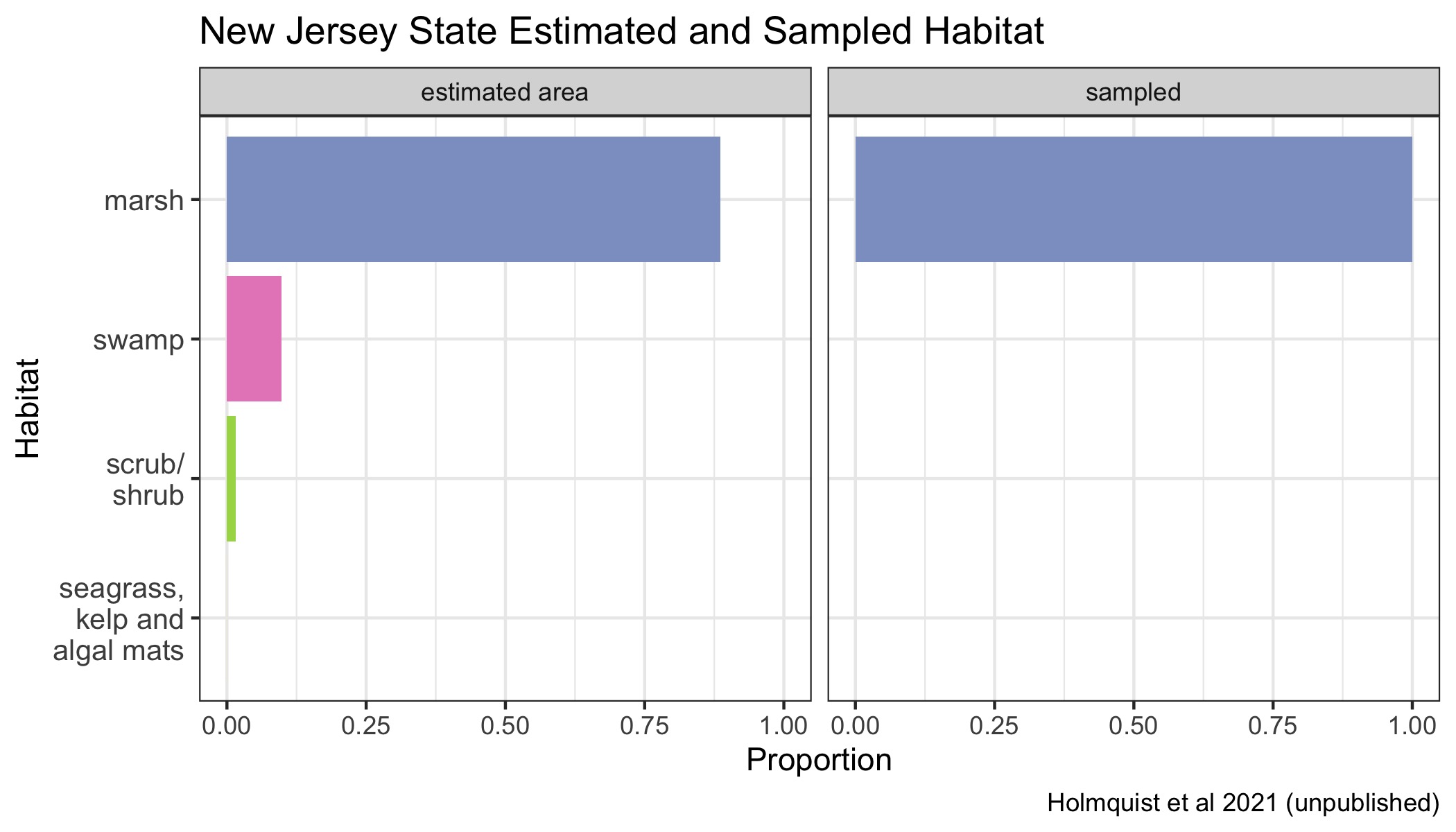
Figure 4.33: Proportions of various Blue Carbon habitats across New Jersey state represented in the dataset in proportion to their estimated area. Seagrasses, kelp beds and algal mats are all combined into a single category, because they are combined in the underlying mapping products.

Table 4.12: Estimated areas and carbon stocks assuming 1 m deposit depth, for select natural tidal wetland ecosystem types in New Jersey. Estimated areas for potential restoration cases.

Class	Area (Ha)	Million Tonnes C
marsh	85142.6	23.0
swamp	9414.8	2.5
scrub/shrub	1500.2	0.4
seagrass, kelp and algal mats	16.5	NA
total natural	96074.1	25.9

4.8.5 Forthcoming Cores

There are many forthcoming cores for New Jersey, contributed largely by Dr. Keryn Gedan of George Washington University. Dr. Nathaniel Weston at Villanova University, also has dated cores with precise elevations for this region currently in prep for data release by the Coastal Carbon Library Network. When this data is released, the number of soil cores from New Jersey will increase by over 500%. All forthcoming cores have associated core elevation, which will improve the overall quality status of soil core data for these states, followed by improvements to spatial and habitat coverage.

4.9 New York State Report

4.9.1 State Overview

New York contains 46 cores or 1.2% of the total number of cores sampled in CONUS. Overall, this state lies at the median relative to other coastal states in CONUS, scoring above the median for quantity, spatial and habitat coverage, but poorly for the quality of available soil cores(Figure 4.34). Because this state contains less than 1% of the coastal wetland habitat in CONUS, the overall quantity of soil cores in the Atlas is representative of this state’s overall contribution of coastal wetlands to CONUS (Figure 4.34A, Figure 4.35). New York’s score can be improved through the collection of more cores that are higher quality with respect to depth, elevation data, and other quality characteristics.

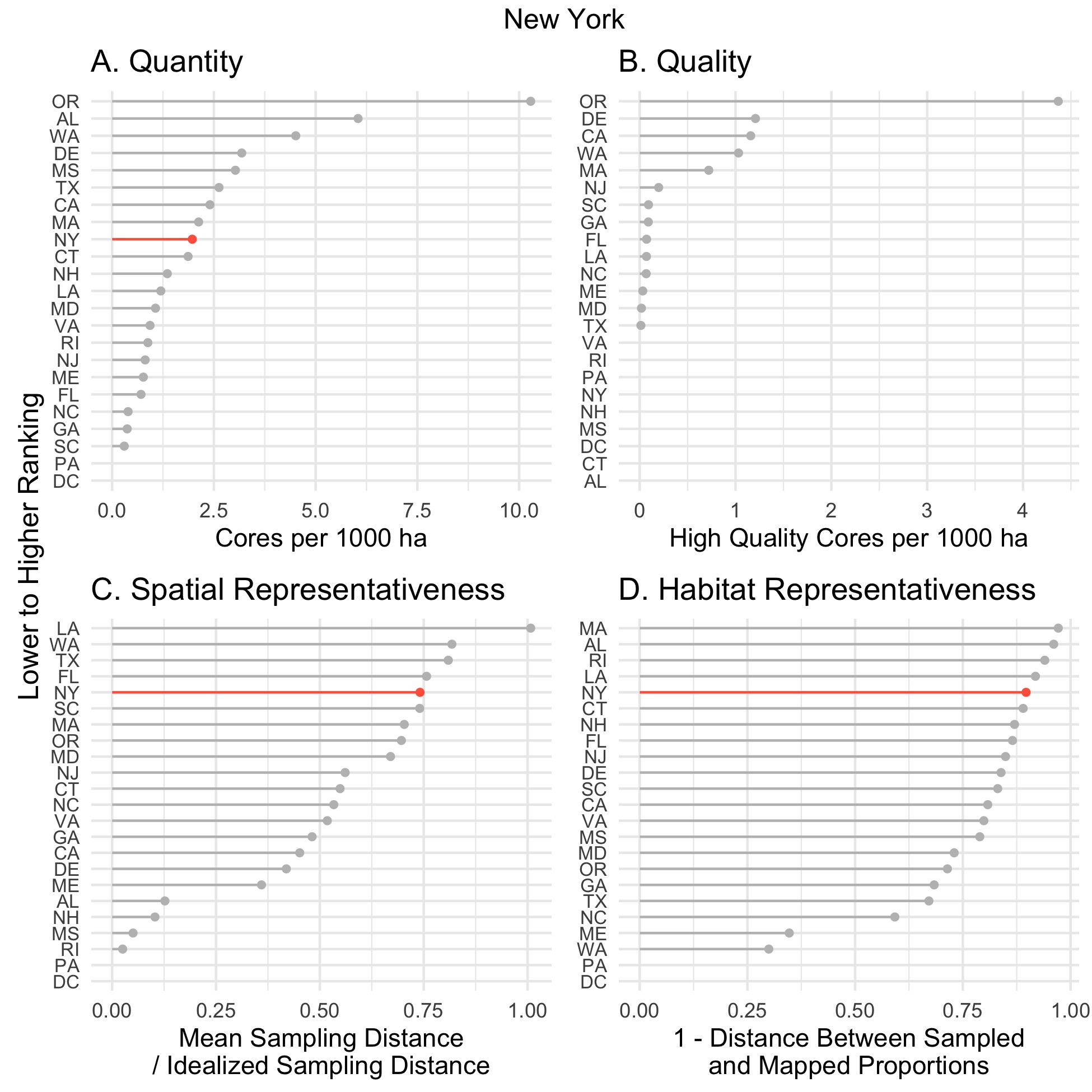
Figure 4.34: State ranking on all four soil Blue Carbon metrics, A. Quantity, B. Quality, C. Spatial Representativeness, D. Habitat Representativeness.

Figure 4.35: State-Level Wetland Contribution

4.9.2 Data Utility and Availability

The quality of the soil core data from New Your is relatively poor (Figure 4.34B). While 82% of cores sampled contain full profiles and can be used for carbon stock assessments, none have enough information to be used in carbon accretion rate assessments or carbon sequestration modeling (Table 4.13).

Table 4.13: Core counts by utility category, and total, for data sources originating from New York

study_id	stocks	dated cores	elevation measurements	other utility	Total	citation
Drake et al. 2015	20	0	0	0	20	(James R. Holmquist et al. 2018; Drake et al. 2015)
Nahlik and Fennessy 2016	0	0	0	8	8	(Nahlik and Fennessy 2016)
Cochran et al. 1998	6	0	0	0	6	(James R. Holmquist et al. 2018; Cochran et al. 1998)
Hill and Anisfeld 2015	6	0	0	0	6	(James R. Holmquist et al. 2018; Hill and Anisfeld 2015)
Merrill 1999	6	0	0	0	6	(James R. Holmquist et al. 2018; Merrill 1999)

4.9.3 Spatial Representativeness

New York exhibits good spatial representativeness of sampling effort (Figure 4.34C, Figure 4.36). A sizable portion of the soil cores are from Long Island, and cores have been collected inland through tidal portions of the Hudson River.

Figure 4.36: Spatial distribution of soil cores across New York state Blue Carbon habitats.

4.9.4 State Habitat Representation

New York scores well for habitat coverage (Figure 4.34D). New York coastal wetland composition is over 80% marsh, with small amounts of swamp, scrub/shrub, and estuarine aquatic bed (EAB; seagrass, kelp bed and algal mat) habitat. However, the samples in our database come entirely from marshes. The absence of samples from scrub/shrub and EAB habitat is offset because the proportional area of these habitats is small but nonetheless New York would benefit from increased sampling of these underrepresented habitats. (Figure 4.37, Table 4.14)

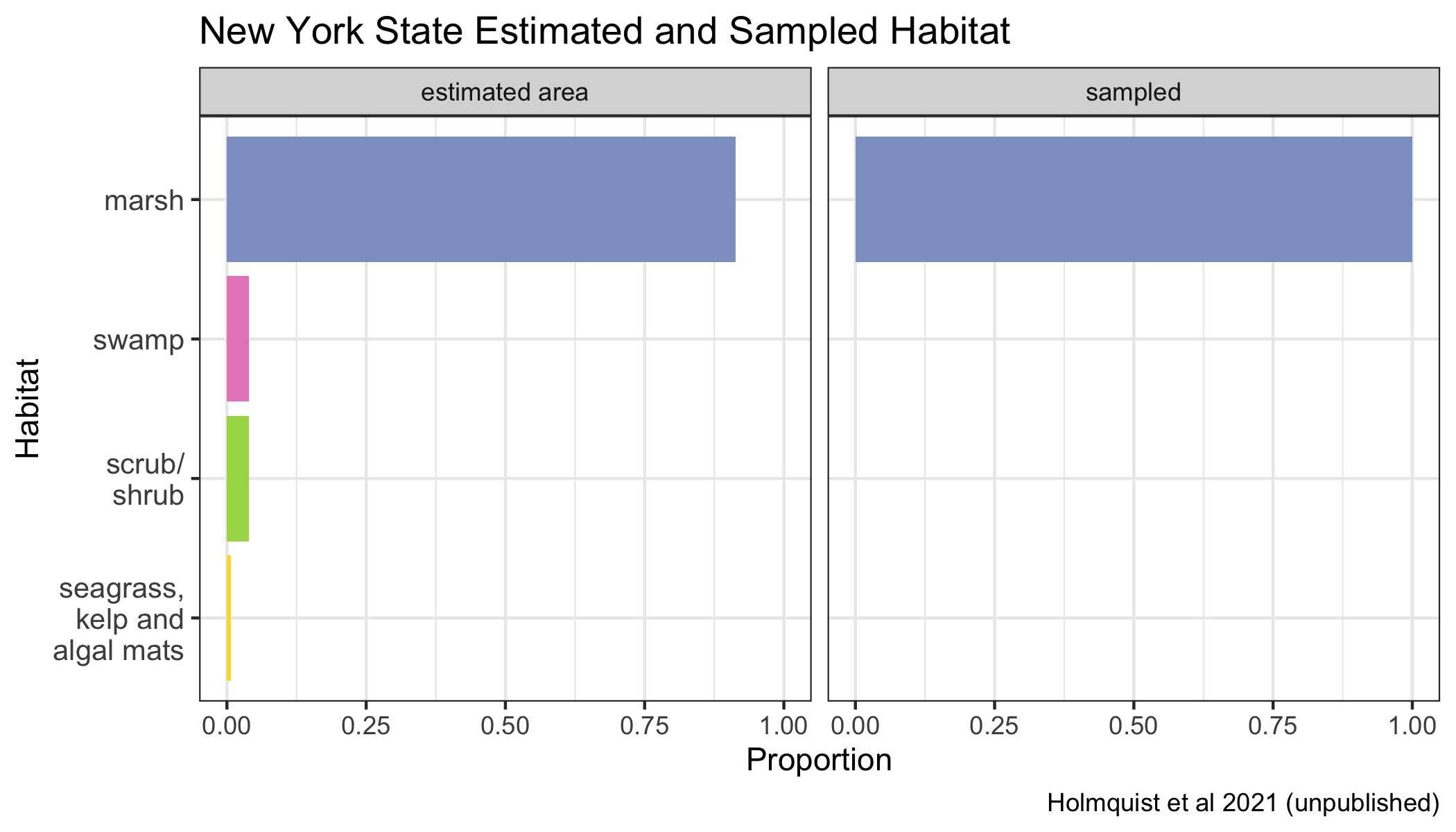
Figure 4.37: Proportions of various Blue Carbon habitats across New York state represented in the dataset in proportion to their estimated area. Seagrasses, kelp beds and algal mats are all combined into a single category, because they are combined in the underlying mapping products.

Table 4.14: Estimated areas and carbon stocks assuming 1 m deposit depth, for select natural tidal wetland ecosystem types in New York. Estimated areas for potential restoration cases.

Class	Area (Ha)	Million Tonnes C
marsh	21351.2	5.8
swamp	933.2	0.3
scrub/shrub	927.3	0.3
seagrass, kelp and algal mats	156.7	NA
total natural	23368.5	6.3

4.9.5 Forthcoming Cores

Cores from the 2015 study lead by Troy Hill report dating information in the literature, however we have been unable to acquire the disaggregated data (Hill and Anisfeld 2015). Dorothy Peteet of NASA and Columbia University also has dated cores from both the Hudson River and Jamaica Bay. These cores are slated for publication via the NEOTOMA data repository, but are still pending.

4.10 Oregon State Report

4.10.1 State Overview

Oregon contains 186 cores or 5% of the total number of tidal wetland cores sampled in CONUS in the Coastal Carbon Atlas. Relative to other coastal states, this state scores in the upper quartile for both quantity and quality metrics, above the median for spatial coverage, and slightly below the median for habitat coverage. The quantity of soil cores sampled in this state is well represented due to a high sampling effort in a state which contains only 0.6% of the total wetland area in CONUS (Figure 4.38A, Figure 4.39). This state’s score can be improved through sampling efforts aimed at increasing spatial and habitat coverage.

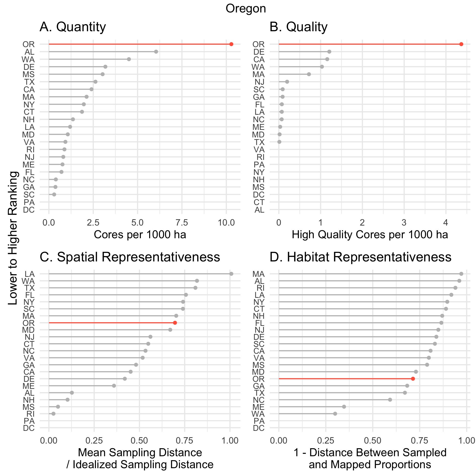
Figure 4.38: State ranking on all four soil Blue Carbon metrics, A. Quantity, B. Quality, C. Spatial Representativeness, D. Habitat Representativeness.

Figure 4.39: State-Level Wetland Contribution

4.10.2 Data Utility and Availability

The utility of the soil core data from Oregon is high relative to other coastal states (Figure 4.38B). Of the cores which are usable for carbon stock assessments, about half can also be used for carbon accretion rate assessments, and roughly a third can be employed for carbon sequestration modeling (Figure 4.40, Table 4.15).

The group led by Craig Cornu and Dr. J Boone Kauffman have grant funding to continue their work, and they have saved core material from the carbon stock data for dating and calculation of carbon burial rates in future studies.

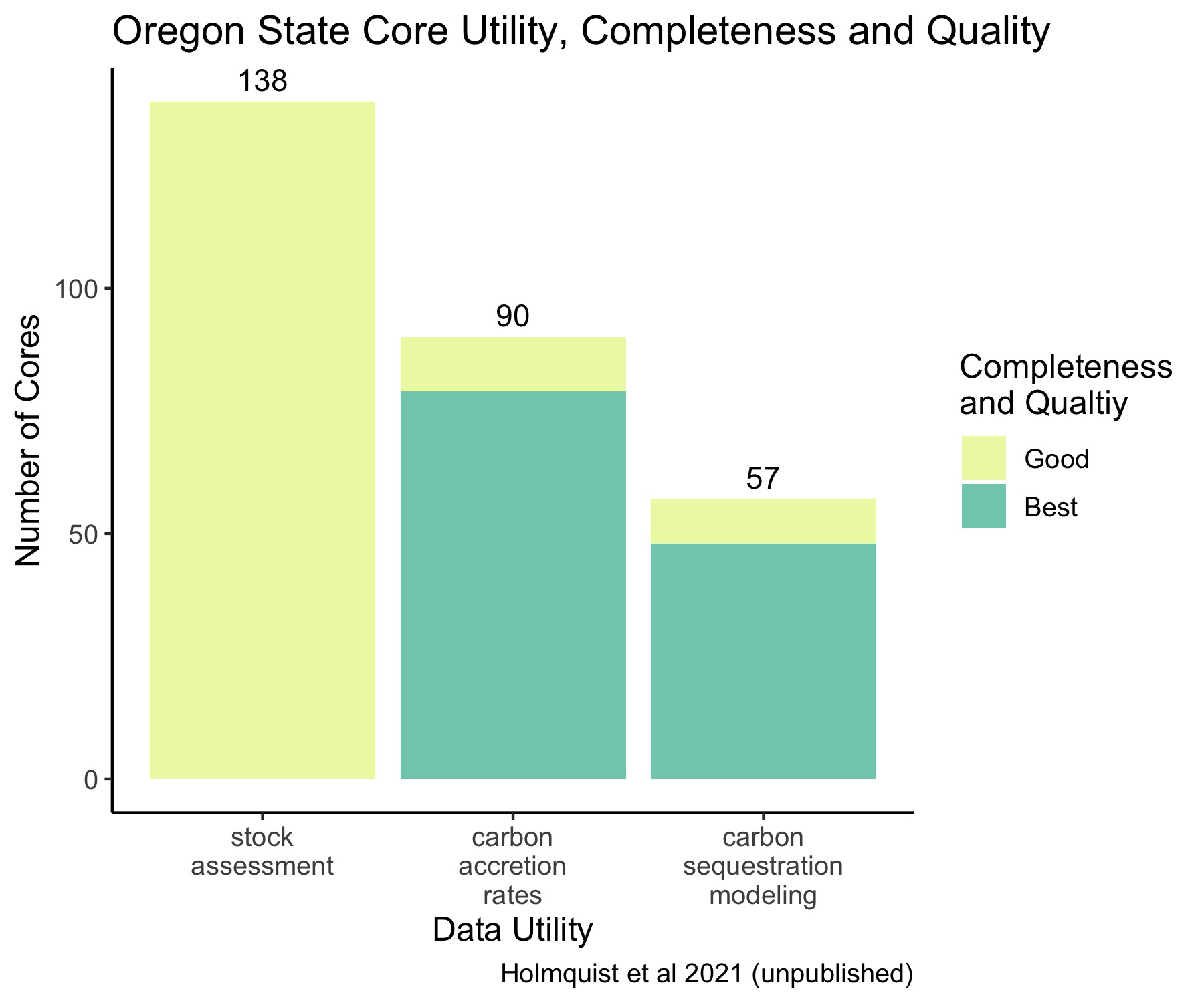
Figure 4.40: Oregon State Core Data Utility, Completeness, and Quality.

Table 4.15: Core counts by utility category, and total, for data sources originating from Oregon

study_id	stocks	dated cores	elevation measurements	other utility	Total	citation
Peck et al. 2020	48	79	48	7	86	(E. Peck, Wheatcroft, and Brophy 2020)
Kauffman et al. 2020	77	0	0	0	77	(J. Boone Kauffman et al. 2020; Kauffman et al. 2020)
Thorne et al. 2015	9	9	9	0	9	(K. M. Thorne et al. 2012)
Larned 2003	0	0	0	6	6	(Fourqurean et al. 2012; Larned 2003)
Hebert et al. 2007	0	0	0	4	4	(Fourqurean et al. 2012; Hebert, Morse, and Eldridge 2007)
Nahlik and Fennessy 2016	2	0	0	0	2	(Nahlik and Fennessy 2016)
Thom 1992	2	2	0	0	2	(Thom 2019, 1992)

4.10.3 Spatial Representativeness

Relative to other coastal states, Oregon scores moderately well for spatial representativeness, leaving room for improvement of spatial coverage (Figure 4.38C, Figure 4.41).

Figure 4.41: Spatial distribution of soil cores across Oregon state Blue Carbon habitats.

4.10.4 State Habitat Representation

This state contains a diversity of Blue Carbon habitats of which over 60% is marsh, followed by scrub/shrub, swamp, and estuarine aquatic bed (EAB; seagrass, kelp bed and algal mat). Swamp and scrub/shrub habitats are underrepresented while there is a bias toward marsh and EAB habitats. Due to the combination of high habitat diversity and the bias toward marsh and EAB habitat, habitat coverage in this state is consequentially low (Figure 4.42, Table 4.16). Habitat representativeness can be improved through increased sampling of swamp and scrub/scrub habitats.

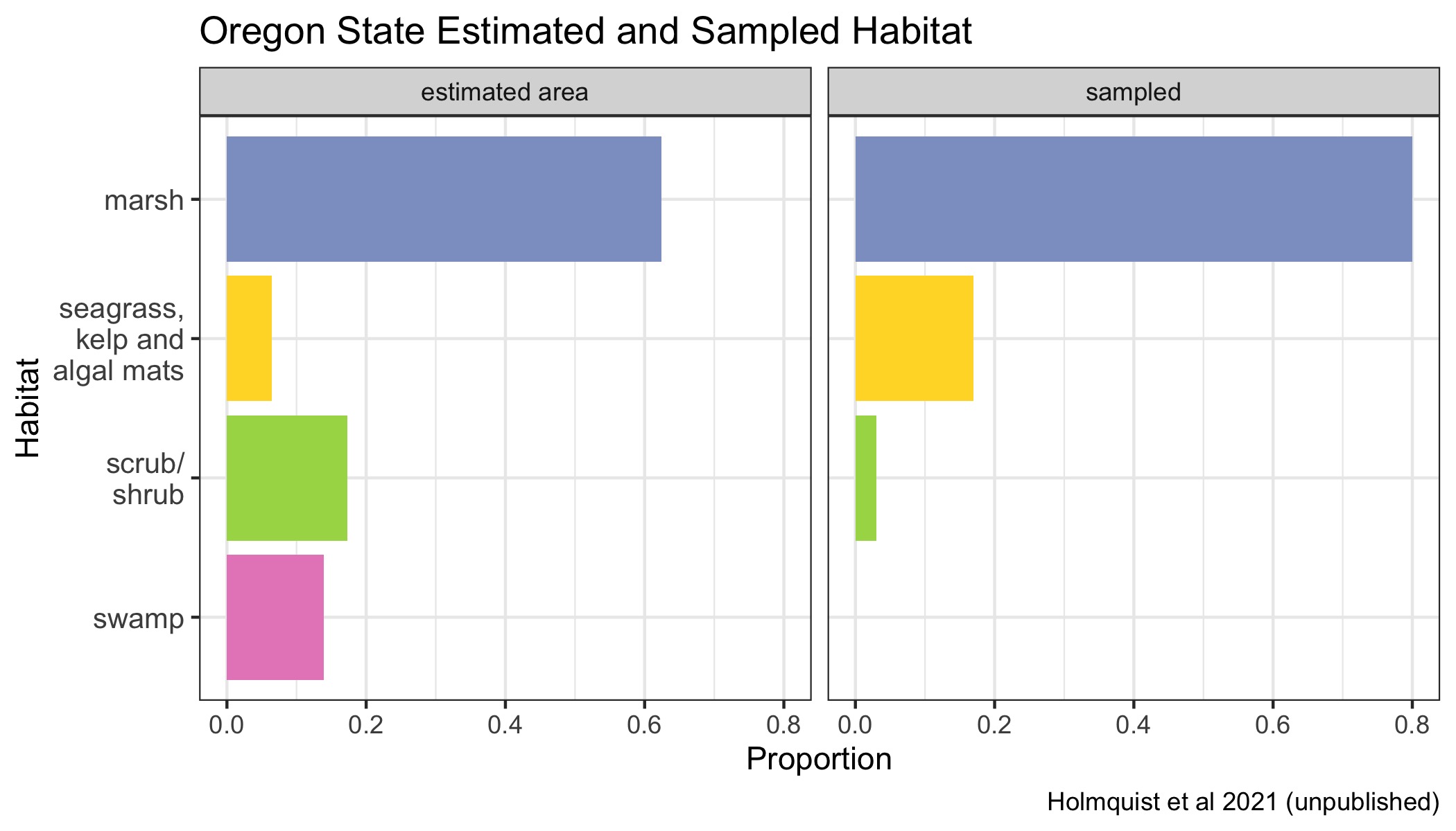
Figure 4.42: Proportions of various Blue Carbon habitats across Oregon state represented in the dataset in proportion to their estimated area. Seagrasses, kelp beds and algal mats are all combined into a single category, because they are combined in the underlying mapping products.

Table 4.16: Estimated areas and carbon stocks assuming 1 m deposit depth, for select natural tidal wetland ecosystem types in Oregon. Estimated areas for potential restoration cases.

Class	Area (Ha)	Million Tonnes C
marsh	11288.4	3.0
scrub/shrub	3127.3	0.8
swamp	2512.1	0.7
seagrass, kelp and algal mats	1158.9	NA
total natural	18086.6	4.6

4.11 Virginia State Report

4.11.1 State Overview

Virginia contains 109 cores or 2.9% of the total number of cores sampled in CONUS. Relative to other coastal states, Virginia scores consistently at or below the median across all metrics, with it’s lowest scores highlighting deficiencies in quantity and quality of soil core data (Figure 4.43). This state contains 4.8% of the wetlands in CONUS, presenting the potential for it’s scores to improve greatly through increased sampling effort and strategic collection of high quality cores in a way that maximizes spatial and habitat coverage (Figure 4.44).

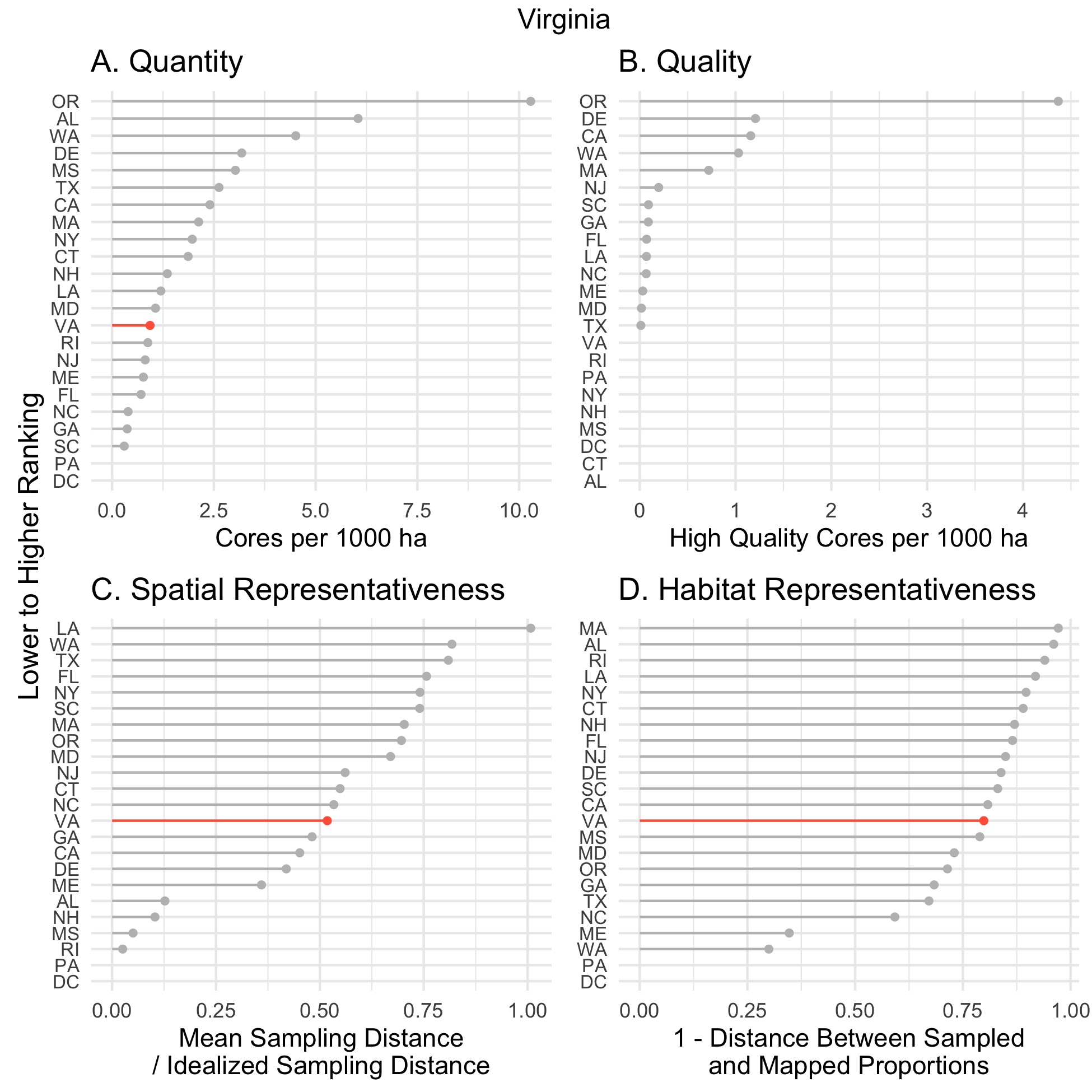
Figure 4.43: State ranking on all four soil Blue Carbon metrics, A. Quantity, B. Quality, C. Spatial Representativeness, D. Habitat Representativeness.

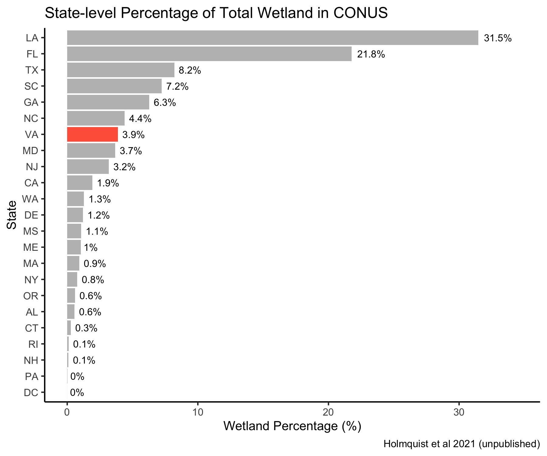
Figure 4.44: State-Level Wetland Contribution

4.11.2 Data Utility and Availability

The utility of the soil core data from Virginia is relatively poor (Figure 4.43B). Almost all of the cores sampled can be used for carbon stock assessments, but none have enough information to be used in carbon accretion rate assessments or carbon sequestration modeling. (Table 4.17)

Table 4.17: Core counts by utility category, and total, for data sources originating from Virginia

study_id	stocks	dated cores	elevation measurements	other utility	Total	citation
Neubauer 2002	60	0	0	0	60	(James R. Holmquist et al. 2018; Neubauer et al. 2002)
Nahlik and Fennessy 2016	24	0	0	0	24	(Nahlik and Fennessy 2016)
Nuttle 1996	13	0	0	0	13	(James R. Holmquist et al. 2018; Nuttle 2018)
McGlathery et al. 2012	8	0	0	0	8	(Fourqurean et al. 2012; McGlathery et al. 2012)
Buzzelli 1998	3	0	0	0	3	(Fourqurean et al. 2012; Buzzelli 1998)
Spivak et al. 2009	0	0	0	1	1	(Fourqurean et al. 2012; AC Spivak et al. 2009)

4.11.3 Spatial Representativeness

Relative to other coastal states, Blue Carbon habitat sampling in Virginia has not been spatially representative (Figure 4.43C, Figure 4.45).

Figure 4.45: Spatial distribution of soil cores across Virginia state Blue Carbon habitats.

4.11.4 State Habitat Representation

Virginia’s Blue Carbon habitats are about 70% marsh and 25% swamp, followed by scrub/shrub and a small amount of estuarine aquatic bed (EAB; seagrass, kelp bed and algal mat). There is a bias toward marsh and EAB in the sampling, while swamp habitat is underrepresented and scrub/shrub is absent. This results in a poor score for habitat representativeness for Virginia That can be improved through increased sampling effort in swamps and scrub/shrub habitat. (Figure 4.46, Table 4.18)

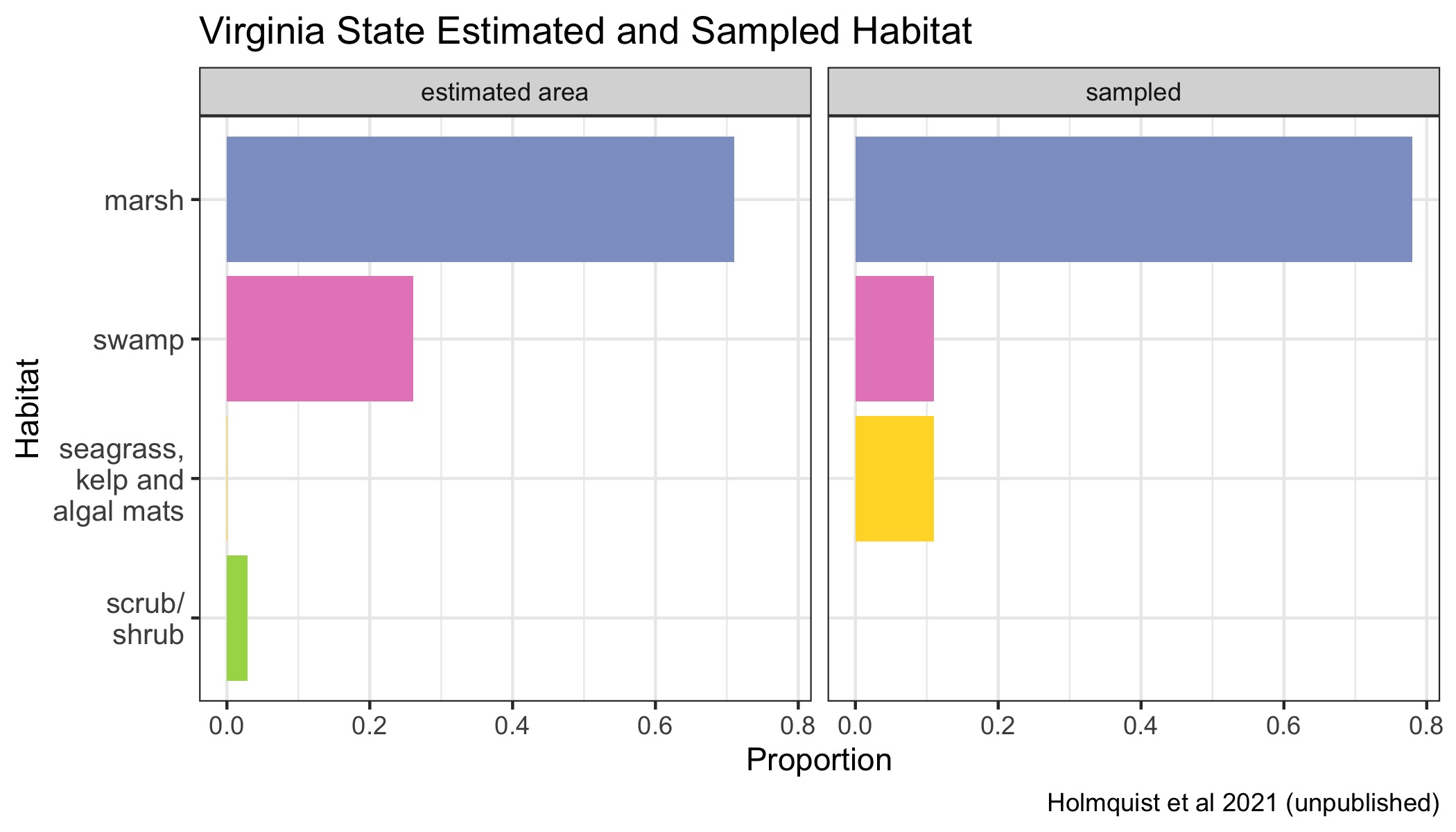
Figure 4.46: Proportions of various Blue Carbon habitats across Virginia represented in the dataset in proportion to their estimated area. Seagrasses, kelp beds and algal mats are all combined into a single category, because they are combined in the underlying mapping products.

Table 4.18: Estimated areas and carbon stocks assuming 1 m deposit depth, for select natural tidal wetland ecosystem types in Virginia. Estimated areas for potential restoration cases.

Class	Area (Ha)	Million Tonnes C
marsh	83080.2	22.4
swamp	30542.2	8.2
scrub/shrub	3362.4	0.9
seagrass, kelp and algal mats	40.9	NA
total natural	117025.7	31.6

4.11.5 Forthcoming cores

Fortunately, there are many new cores forthcoming out of Virginia, largely contributed by Dr. Keryn Gedan of George Washington University. Dr. Nathaniel Weston is also in the process of publishing 6 cores, 3 for the York River and 3 for the James River, all of which will be the highest quality. When these data are released the number of soil cores from Virginia will increase by over 380%.

4.12 Washington State Report

4.12.1 State Overview

Washington state contains 175 cores or 4.7% of all tidal wetland cores sampled in CONUS that are available through the Atlas. Relative to other coastal states, the soil core data of this state is comparatively high quality and well-represented in quantity and spatial coverage, but falls below the median for habitat coverage (Figure 4.47). Washington state scores well overall because there are a large number of high-quality cores available for a state that contains a small fraction of CONUS Blue Carbon habitats (1.3% of CONUS coastal wetland area) (Figure 4.47A, Figure 4.48). This state’s score can be improved through sampling efforts aimed at increasing habitat coverage.

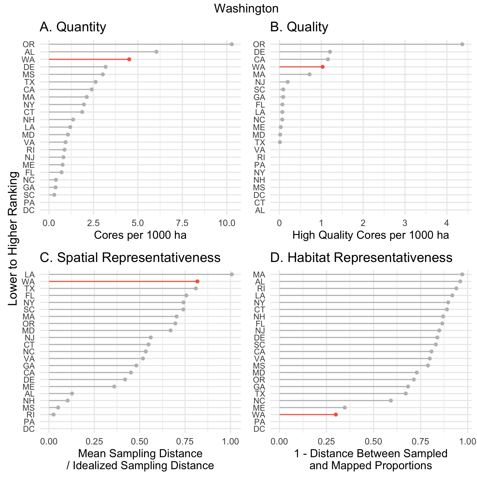
Figure 4.47: State ranking on all four soil Blue Carbon metrics, A. Quantity, B. Quality, C. Spatial Representativeness, D. Habitat Representativeness.

Figure 4.48: State-Level Wetland Contribution

4.12.2 Data Utility and Availability

The quality of the soil core data from Washington state is high relative to other states, with many A1-level cores per 1,000 ha of wetland (Figure 4.47B). Almost all cores can be used for carbon stock assessments, 36% of which are useful for carbon accretion rate assessments and 28% of which are useful for carbon sequestration modeling (Figure 4.49, Table 4.19).

The group led by Craig Cornu and Dr. J Boone Kauffman have grant funding to continue their work, and they have saved core material from the carbon stock data for dating and calculation of carbon burial rates in future studies.

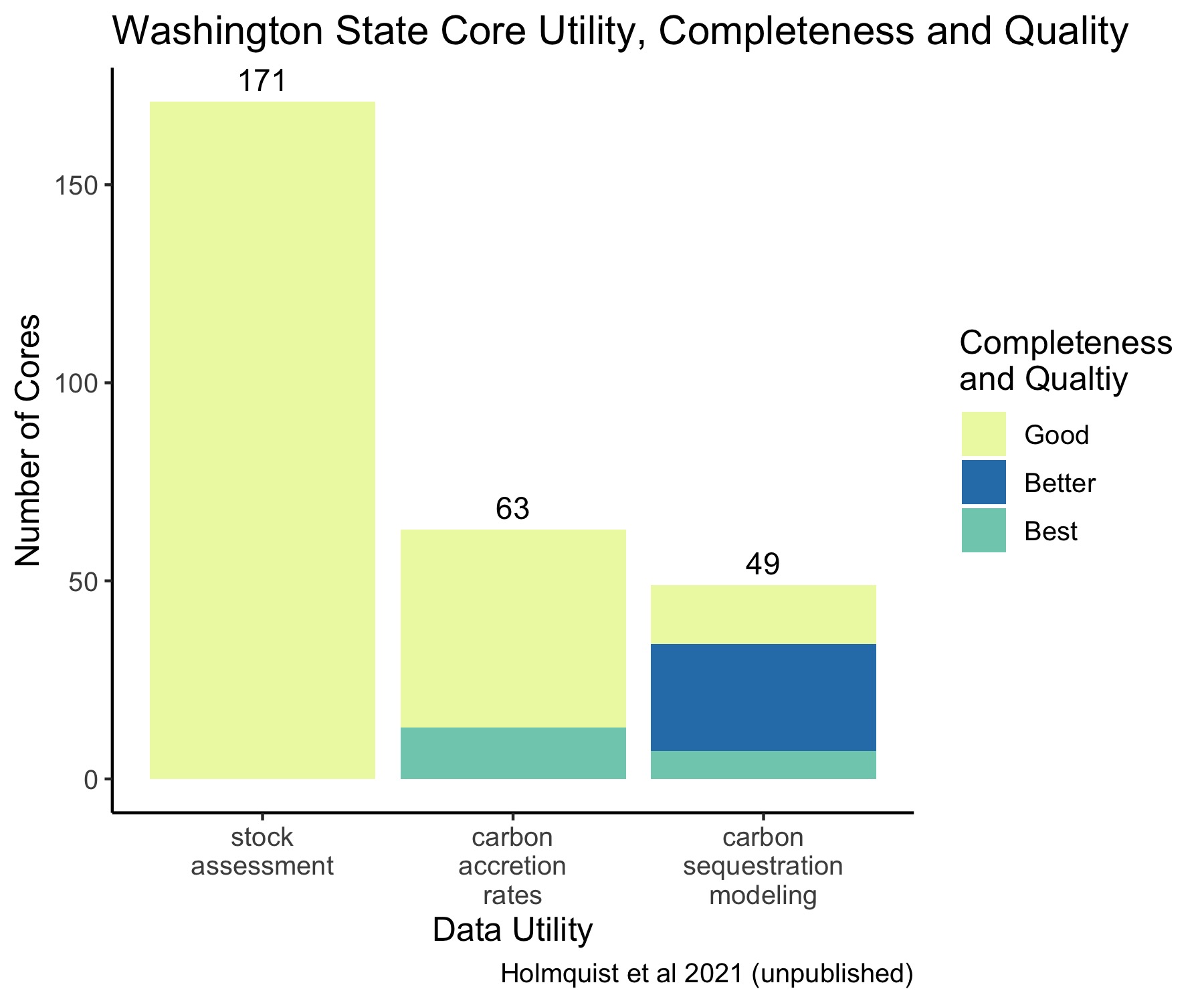
Figure 4.49: Washington State Core Data Utility, Completeness, and Quality.

Table 4.19: Core counts by utility category, and total, for data sources originating from Washington

study_id	stocks	dated cores	elevation measurements	other utility	Total	citation
Kauffman et al. 2020	72	0	0	0	72	(J. Boone Kauffman et al. 2020; Kauffman et al. 2020)
Poppe and Rybczyk 2019	26	15	15	0	26	(Katrina Poppe and Rybczyk 2019; KL Poppe and Rybczyk 2019)
Poppe et al. 2019	23	12	12	0	23	(Katrina Poppe and Rybczyk 2019; Crooks et al. 2014)
Thorne et al. 2015	15	15	15	0	15	(K. M. Thorne et al. 2012)
Drexler et al. 2019	12	6	0	0	12	(Drexler et al. 2019)
Thom 1992	8	8	0	0	8	(Thom 2019, 1992)
Nahlik and Fennessy 2016	7	0	0	0	7	(Nahlik and Fennessy 2016)
Poppe and Rybczyk 2018	7	7	7	0	7	(Katrina Poppe and Rybczyk 2019; KL Poppe and Rybczyk 2018; KL Poppe 2015)
Peck et al. 2020	0	0	0	4	4	(E. Peck, Wheatcroft, and Brophy 2020)
Kairis and Rybczyk 2010	1	0	0	0	1	(Fourqurean et al. 2012; Kairis and Rybczyk 2010)

4.12.3 Spatial Representativeness

Relative to other coastal states, this state scores moderately well for spatial representativeness, but there is still room for improvement of spatial coverage (Figure 4.47C, Figure 4.50).

Figure 4.50: Spatial distribution of soil cores across Washington state Blue Carbon habitats.

4.12.4 State Habitat Representation

Washington state contains a wide diversity of Blue Carbon habitats. Setting it apart from other states, Washington’s Blue Carbon habitat composition is dominated by estuarine aquatic bed (EAB; seagrass, kelp bed and algal mat; 55%) compared to marsh (30%), followed by swamp, and scrub/shrub (Figure 4.51). There is a sampling bias toward marsh habitat whereas EAB is vastly underrepresented. At a smaller scale in terms of area, there is a bias toward swamp habitat while scrub/shrub is underrepresented. Habitat coverage is a weak spot for this state, but can be improved through increased sampling of EAB and scrub/scrub habitats. (Table 4.20)

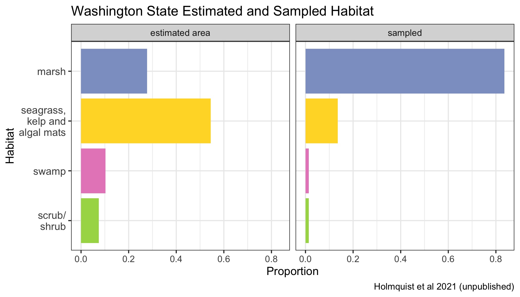
Figure 4.51: Proportions of various Blue Carbon habitats across Washington state represented in the dataset in proportion to their estimated area. Seagrasses, kelp beds and algal mats are all combined into a single category, because they are combined in the underlying mapping products.

Table 4.20: Estimated areas and carbon stocks assuming 1 m deposit depth, for select natural tidal wetland ecosystem types in Washington state. Estimated areas for potential restoration cases.

Class	Area (Ha)	Million Tonnes C
seagrass, kelp and algal mats	21140.2	NA
marsh	10767.6	2.9
swamp	3985.1	1.1
scrub/shrub	2893.0	0.8
total natural	38785.9	4.8

4.13 Local Scale Mapping Improvements

4.13.1 Status of Seagrass Mapping

The national scale maps used for our habitat area estimates do not map seagrasses specifically, but instead lump together seagrasses, algal mats, and kelp beds under a single Estuarine Aquatic Bed classification. For this reason, we provide some insights on states where there is are more detailed seagrass mapping programs.

We reached out to Jon Lefcheck of SERC for his understanding of the current state of seagrass maps for the United States. The most comprehensive seagrass map on a US national-scale is NOAA’s Marine Cadastre, which is a resource that was jointly developed by NOAA and BOEM to support renewable energy projects and other marine-related initiatives. One of many layers in Marine Cadastre is seagrass. Data on the presence and location of seagrasses was compiled from many state and local sources. However, the sources are not well documented at present because the map is not linked to the data sources and the sources are not linked to the raw data as in the Coastal Carbon Atlas. Marine Cadastre also appears to lack an evaluation of data quality.

Marine Cadastre is updated every two years, with the seagrass layer being last updated in March 2020. However, it does not have two notable regional seagrass mapping efforts in progress. One is a seagrass map of Florida by Luis Lizcano-Sandoval, a graduate student at the University of South Florida. The other effort is from the Chesapeake Bay Submerged Aquatic Vegetation mapping program which is current through 2020.

There is interest in improving seagrass maps. Presently Jon Lefcheck is discussing with Marine Cadastre the possibility of building a comprehensive registry for seagrass maps modeled on National Wetlands Inventory maps. Jon and Luis Lizcano-Sandoval are considering applying his methods (based on machine learning of remotely sensed data) to Puerto Rico as part of a NOAA-led seagrass monitoring program in summer 2021. Finally, Jon is collaborating with Jim Fourqurean at Florida International University on an effort to collate all seagrass datasets for an international synthesis effort. There is a dedicated post-doc in Jim’s lab to advance that project. Jon is presently collaborating with Pew on the National Coordination Alliance for SAV Enhancement (Aaron Kornbluth) and on Pew international programs related to seagrass ecosystems (Stacy Baez and Katelyn Theuerkauf).

4.13.2 Local Improvements in Former Wetland Mapping

Other locally specific products include a west coast map by Brophy et al. (2019) which has some improved functionality for mapping eroded wetlands, and some regional datasets which have alternative methods for mapping impoundments. Our mapping products do a very similar layer of wetland, tidal elevation, and land cover change mapping with a few minor methodological differences at the national level. Our products do not integrate maps of historical wetlands coverage based on detailed shoreline surveys starting in the 1840’s. This improvement is only available for CA, WA, and OR.

4.13.3 Local Impoundment Datasets

There is one additional local dataset for mapping impoundments that we are aware of, which is the Maine Tidal Restriction Atlas. It has detailed information, but is point based, meaning it does not map the upstream hydrology or account for areas of wetlands affected by impoundments.

References

Arriola, Jill M., and Jaye E. Cable. 2017. “Variations in Carbon Burial and Sediment Accretion Along a Tidal Creek in a Florida Salt Marsh.” Limnology and Oceanography 62 (November): S15–28. https://doi.org/10.1002/lno.10652.

Boyd, Brandon M., Christopher K. Sommerfield, and Tracy Elsey-Quirk. 2017. “Hydrogeomorphic Influences on Salt Marsh Sediment Accumulation and Accretion in Two Estuaries of the U.S. Mid-Atlantic Coast.” Marine Geology 383: 132–45. https://doi.org/10.1016/j.margeo.2016.11.008.

Boyd, Brandon, Christopher K. Sommerfield, Tracy Quirk, and Viktoria Unger. 2019. “Dataset: Accretion and Sediment Accumulation in Impounded and Unimpounded Marshes in the Delaware Estuary and Barnegat Bay.” The Smithsonian Institution. https://doi.org/10.25573/data.9747065.

Breithaupt, Joshua L., Joseph M. Smoak, Victor H. Rivera-Monroy, Edward Castañeda-Moya, Ryan P. Moyer, Marc Simard, and Christian J. Sanders. 2017. “Partitioning the Relative Contributions of Organic Matter and Mineral Sediment to Accretion Rates in Carbonate Platform Mangrove Soils.” Marine Geology 390 (August): 170–80. https://doi.org/10.1016/j.margeo.2017.07.002.

Breithaupt, Joshua L., Joseph M. Smoak, Christian J. Sanders, and Thomas J. Smith III. 2019. “Dataset: Temporal Variability of Carbon and Nutrient Burial, Sediment Accretion, and Mass Accumulation over the Past Century in a Carbonate Platform Mangrove Forest of the Florida Everglades.” The Smithsonian Institution. https://doi.org/10.25573/serc.11310926.

Breithaupt, Joshua L, Joseph M Smoak, Thomas J Smith III, and Christian J Sanders. 2014. “Temporal Variability of Carbon and Nutrient Burial, Sediment Accretion, and Mass Accumulation over the Past Century in a Carbonate Platform Mangrove Forest of the Florida Everglades.” Journal of Geophysical Research: Biogeosciences 119 (10): 2032–48. https://doi.org/10.1002/2014JG002715.

Breithaupt, Joshua L., Smoak, Joseph M., Bianchi, Thomas S., Vaughn, et al. 2020. “Dataset: Increasing Rates of Carbon Burial in Southwest Florida Coastal Wetlands.” The Smithsonian Institution. https://doi.org/10.25573/data.9894266.

Brophy, Laura S, Correigh M Greene, Van C Hare, Brett Holycross, Andy Lanier, Walter N Heady, Kevin O’Connor, Hiroo Imaki, Tanya Haddad, and Randy Dana. 2019. “Insights into Estuary Habitat Loss in the Western United States Using a New Method for Mapping Maximum Extent of Tidal Wetlands.” PloS One 14 (8): e0218558.

Buffington, Kevin, Christopher Janousek, Karen Thorne, and Bruce Dugger. 2020. “Dataset: Carbon Stocks and Accretion Rates for Wetland Sediment at Miner Slough, Sacramento-San Joaquin Delta, California.” The Smithsonian Institution. https://doi.org/10.25573/SERC.11968740.

BURNS, STEPHEN J., and PETER K. SWART. 1992. “Diagenetic Processes in Holocene Carbonate Sediments: Florida Bay Mudbanks and Islands.” Sedimentology 39 (2): 285–304. https://doi.org/10.1111/j.1365-3091.1992.tb01039.x.

Buzzelli, Christopher P. 1998. “Dynamic Simulation of Littoral Zone Habitats in Lower Chesapeake Bay. I. Ecosystem Characterization Related to Model Development.” Estuaries 21 (4): 659–72. https://doi.org/10.2307/1353271.

Cahoon, Donald R, Lynch, and James C. 1997. “Vertical Accretion and Shallow Subsidence in a Mangrove Forest of Southwestern Florida, USA.” Mangroves and Salt Marshes 1 (3): 173–86. https://doi.org/10.1023/A:1009904816246.

Callaway, John C., Evyan L. Borgnis, R. Eugene Turner, and Charles S. Milan. 2012a. “Carbon Sequestration and Sediment Accretion in San Francisco Bay Tidal Wetlands.” Estuaries and Coasts 35 (5): 1163–81. https://doi.org/10.1007/s12237-012-9508-9.

Callaway, John C., Evyan L. Borgnis, R. Eugene Turner, and Charles S. Milan. 2019. “Dataset: Carbon Sequestration and Sediment Accretion in San Francisco Bay Tidal Wetlands.” The Smithsonian Institution. https://doi.org/10.25573/data.9693251.

Callaway, JC, DeLaune, RD, Patrick Jr, and WH. 1997. “Sediment Accretion Rates from Four Coastal Wetlands Along the Gulf of Mexico.” Journal of Coastal Research 13 (1): 181–91.

Chen, Ronghua, and Robert R. Twilley. 1999. “A Simulation Model of Organic Matter and Nutrient Accumulation in Mangrove Wetland Soils.” Biogeochemistry 44 (January): 93–118. https://doi.org/10.1007/bf00993000.

Chmura, Gail L., Shimon C. Anisfeld, Donald R. Cahoon, and James C. Lynch. 2003. “Global Carbon Sequestration in Tidal, Saline Wetland Soils.” Global Biogeochemical Cycles 17 (4): n/a–. https://doi.org/10.1029/2002gb001917.

Cochran, J. K., D. J. Hirschberg, J. Wang, and C. Dere. 1998. “Atmospheric Deposition of Metals to Coastal Waters (Long Island Sound, New York U.S.A.): Evidence from Saltmarsh Deposits.” Estuarine, Coastal and Shelf Science 46 (4): 503–22. https://doi.org/10.1006/ecss.1997.0299.

Crooks, S, J Rybczyk, K O‘Connell, D L Devier, K Poppe, and S Emmett-Mattox. 2014. “Coastal Blue Carbon Opportunity Assessment for the Snohomish Estuary: The Climate Benefits of Estuary Restoration.” Restore America’s Estuaries.

Doughty, Cheryl L., J. Adam Langley, Wayne S. Walker, Ilka C. Feller, Ronald Schaub, and Samantha K. Chapman. 2016. “Mangrove Range Expansion Rapidly Increases Coastal Wetland Carbon Storage.” Estuaries and Coasts 39 (May): 385–96. https://doi.org/10.1007/s12237-015-9993-8.

Doughty, Cheryl, J. Adam Langley, Wayne Walker, Ilka C. Feller, Ronald Schaub, and Samantha Chapman. 2019. “Mangroves Marching Northward: The Impacts of Rising Seas and Temperatures on Ecosystems at Kennedy Space Center.” The Smithsonian Institution. https://doi.org/10.25573/data.9695918.v1.

Drake, Katherine, Holly Halifax, Susan C. Adamowicz, and Christopher Craft. 2015. “Carbon Sequestration in Tidal Salt Marshes of the Northeast United States.” Environmental Management 56 (4): 998–1008. https://doi.org/10.1007/s00267-015-0568-z.

Drexler, Judith Z., Christian S. de Fontaine, and Thomas A. Brown. 2009. “Peat Accretion Histories During the Past 6,000 Years in Marshes of the Sacramento–San Joaquin Delta, CA, USA.” Estuaries and Coasts 32 (5): 871–92. https://doi.org/10.1007/s12237-009-9202-8.

Drexler, Judith Z., Isa Woo, Christopher C. Fuller, and Glynnis Nakai. 2019. “Carbon Accumulation and Vertical Accretion in a Restored Versus Historic Salt Marsh in Southern Puget Sound, Washington, United States.” Restoration Ecology, September. https://doi.org/10.1111/rec.12941.

El Shahat Sedik Keshta, Amr. 2017. “HYDROLOGY, SOIL REDOX, AND PORE-WATER IRON REGULATE CARBON CYCLING IN NATURAL AND RESTORED TIDAL FRESHWATER WETLANDS IN THE CHESAPEAKE BAY, MARYLAND, USA.” PhD thesis, University of Maryland. https://doi.org/10.13016/M2S756M71.

El Shahat Sedik Keshta, Amr, Stephanie A. Yarwood, and Andrew H. Baldwin. 2020. “Dataset: Soil Redox and Hydropattern Control Soil Carbon Stocks Across Different Habitats in Tidal Freshwater Wetlands in a Sub-Estuary of the Chesapeake Bay.” The Smithsonian Institution. https://doi.org/10.25573/serc.13187549.

Ensign, Scott H., Gregory B. Noe, Cliff R. Hupp, and Katherine J. Skalak. 2015. “Head-of-Tide Bottleneck of Particulate Material Transport from Watersheds to Estuaries.” Geophysical Research Letters 42 (24): 10, 671–10, 679. https://doi.org/10.1002/2015gl066830.

Fourqurean, James W., Carlos M. Duarte, Hilary Kennedy, Núria Marbà, Marianne Holmer, Miguel Angel Mateo, Eugenia T. Apostolaki, et al. 2012. “Seagrass Ecosystems as a Globally Significant Carbon Stock.” Nature Geoscience 5 (7): 505–9. https://doi.org/10.1038/ngeo1477.

Fourqurean, James W., Meredith F. Muth, and Joseph N. Boyer. 2010. “Epiphyte Loads on Seagrasses and Microphytobenthos Abundance Are Not Reliable Indicators of Nutrient Availability in Oligotrophic Coastal Ecosystems.” Marine Pollution Bulletin 60 (7): 971–83. https://doi.org/10.1016/j.marpolbul.2010.03.003.

Gerlach, Matthew J., Simon E. Engelhart, Andrew C. Kemp, Ryan P. Moyer, Joseph M. Smoak, Christopher E. Bernhardt, and Niamh Cahill. 2017. “Reconstructing Common Era Relative Sea-Level Change on the Gulf Coast of Florida.” Marine Geology 390 (August): 254–69. https://doi.org/10.1016/j.margeo.2017.07.001.

Giblin, Anne, Inke Forbrich, and Plum Island Ecosystems LTER. 2018. “PIE LTER High Marsh Sediment Chemistry and Activity Measurements, Nelson Island Creek Marsh, Rowley, MA.” Environmental Data Initiative. https://doi.org/10.6073/pasta/d1d5cbf87602ccf51de30b87b8e46d01.

Gonneea, Meagan, Kevin Kroeger, and Jennifer O’Keefe-Suttles. 2018. “Collection, Analysis, and Age-Dating of Sediment Cores from Salt Marshes on the South Shore of Cape Cod, Massachusetts, from 2013 Through 2014.” U.S. Geological Survey. https://doi.org/10.5066/f7h41qpp.

Grady, John R. 1981. “Properties of Sea Grass and Sand Flat Sediments from the Intertidal Zone of St. Andrew Bay, Florida.” Estuaries 4 (December): 335. https://doi.org/10.2307/1352158.

Hebert, Andrew B., John W. Morse, and Peter M. Eldridge. 2007. “Small-Scale Heterogeneity in the Geochemistry of Seagrass Vegetated and Non-Vegetated Estuarine Sediments: Causes and Consequences.” Aquatic Geochemistry 13 (1): 19–39. https://doi.org/10.1007/s10498-006-9007-3.

Hill, Troy D., and Shimon C. Anisfeld. 2015. “Coastal Wetland Response to Sea Level Rise in Connecticut and New York.” Estuarine, Coastal and Shelf Science 163 (September): 185–93. https://doi.org/10.1016/j.ecss.2015.06.004.

Holmquist, James R., Lisamarie Windham-Myers, Norman Bliss, Stephen Crooks, James T. Morris, J. Patrick Megonigal, Tiffany Troxler, et al. 2018. “Accuracy and Precision of Tidal Wetland Soil Carbon Mapping in the Conterminous United States: Public Soil Carbon Data Release.” Smithsonian Research Online. https://doi.org/10.25572/ccrcn/10088/35684.

J. Boone Kauffman, Leila Giovanonni, James Kelly, Nicholas Dunstan, Amy Borde, Heida Diefenderfer, Craig Cornu, Christopher Janousek, Jude Apple, and Laura Brophy. 2020. “Dataset: Carbon Stocks in Seagrass Meadows, Emergent Marshes, and Forested Tidal Swamps of the Pacific Northwest.” The Smithsonian Institution. https://doi.org/10.25573/serc.12640172.

Johnson, Beverly J., Karen A. Moore, Charlotte Lehmann, Curtis Bohlen, and Thomas A. Brown. 2007. “Middle to Late Holocene Fluctuations of C3 and C4 Vegetation in a Northern New England Salt Marsh, Sprague Marsh, Phippsburg Maine.” Organic Geochemistry 38 (3): 394–403. https://doi.org/10.1016/j.orggeochem.2006.06.006.

Kairis, Peter A., and John M. Rybczyk. 2010. “Sea Level Rise and Eelgrass (Zostera marina) Production: A Spatially Explicit Relative Elevation Model for Padilla Bay, WA.” Ecological Modelling 221 (7): 1005–16. https://doi.org/10.1016/j.ecolmodel.2009.01.025.

Kauffman, J. Boone, Leila Giovanonni, James Kelly, Nicholas Dunstan, Amy Borde, Heida Diefenderfer, Craig Cornu, Christopher Janousek, Jude Apple, and Laura Brophy. 2020. “Total Ecosystem Carbon Stocks at the Marine-Terrestrial Interface: Blue Carbon of the Pacific Northwest Coast, United States.” Global Change Biology, October. https://doi.org/10.1111/gcb.15248.

Kemp, Andrew C., Christopher K. Sommerfield, Christopher H. Vane, Benjamin P. Horton, Simon Chenery, Shimon Anisfeld, and Daria Nikitina. 2012. “Use of Lead Isotopes for Developing Chronologies in Recent Salt-Marsh Sediments.” Quaternary Geochronology 12 (October): 40–49. https://doi.org/10.1016/j.quageo.2012.05.004.

———. 2020. “Dataset: Use of Lead Isotopes for Developing Chronologies in Recent Salt-Marsh Sediments.” The Smithsonian Institution. https://doi.org/10.25573/serc.11569419.

Larned, ST. 2003. “Effects of the Invasive, Nonindigenous Seagrass Zostera japonica on Nutrient Fluxes Between the Water Column and Benthos in a NE Pacific Estuary.” Marine Ecology Progress Series 254: 69–80. https://doi.org/10.3354/meps254069.

Lewis, Michael A., Darrin D. Dantin, Cynthia A. Chancy, Kathryn C. Abel, and Christopher G. Lewis. 2007. “Florida Seagrass Habitat Evaluation: A Comparative Survey for Chemical Quality.” Environmental Pollution 146 (1): 206–18. https://doi.org/10.1016/j.envpol.2006.04.041.

Luk, Sheron Y., Katherine Todd-Brown, Meagan Eagle, Ann P. McNichol, Jonathan Sanderman, Kelsey Gosselin, and Amanda C. Spivak. 2021. “Soil Organic Carbon Development and Turnover in Natural and Disturbed Salt Marsh Environments.” Geophysical Research Letters 48 (2). https://doi.org/10.1029/2020gl090287.

Luk, Sheron Y, Amanda C Spivak, Meagan J Eagle, and Jennifer A O’keefe Suttles. 2020. “Collection, Analysis, and Age-Dating of Sediment Cores from a Salt Marsh Platform and Ponds, Rowley, Massachusetts, 2014-15.” U.S. Geological Survey. https://doi.org/10.5066/p9hiowkt.

Marchio, Daniel, Michael Savarese, Brian Bovard, and William Mitsch. 2016. “Carbon Sequestration and Sedimentation in Mangrove Swamps Influenced by Hydrogeomorphic Conditions and Urbanization in Southwest Florida.” Forests 7 (6): 116. https://doi.org/10.3390/f7060116.

McGlathery, KJ, LK Reynolds, LW Cole, RJ Orth, SR Marion, and A Schwarzschild. 2012. “Recovery Trajectories During State Change from Bare Sediment to Eelgrass Dominance.” Marine Ecology Progress Series 448 (February): 209–21. https://doi.org/10.3354/meps09574.

Merrill, J Z. 1999. “Tidal Freshwater Marshes as Nutrient Sinks: Particulate Nutrient Burial and Denitrification.” PhD thesis, University of Maryland, College Park. https://elibrary.ru/item.asp?id=5305392.

Messerschmidt, Tyler C., and Matthew L. Kirwan. 2020. “Dataset: Soil Properties and Accretion Rates of C3 and C4 Marshes at the Global Change Research Wetland, Edgewater, Maryland.” The Smithsonian Institution. https://doi.org/10.25573/SERC.11914140.

Nahlik, Amanda M., and Siobhan Fennessy. 2016. “Carbon Storage in US Wetlands.” Nature Communications, December. https://doi.org/10.1038/ncomms13835.

Neubauer, S. C., I. C. Anderson, J. A. Constantine, and S. A. Kuehl. 2002. “Sediment Deposition and Accretion in a Mid-Atlantic (U.S.A.) Tidal Freshwater Marsh.” Estuarine, Coastal and Shelf Science 54 (4): 713–27. https://doi.org/10.1006/ecss.2001.0854.

Nuttle, William. 2018. “Marsh Sediment Dynamics and Organic Matter Survey VCR/LTER 1987-1988.” Environmental Data Initiative. https://doi.org/10.6073/pasta/2c67d3744ef1e10138ca010066c0cfb5.

Orem, W. H., Holmes, C. W., Kendall, C., Lerch, et al. 1999. “Geochemistry of Florida Bay Sediments: Nutrient History at Five Sites in Eastern and Central Florida Bay.” Journal of Coastal Research 15. https://www.jstor.org/stable/4299024.

Osland, Michael J., J. B. Grace, C. L. Stagg, R. H. Day, S. B. Hartley, N. M. Enwright, and C. A Gabler. 2016. “U.S. Gulf of Mexico Coast (TX, MS, AL, and FL) Vegetation, Soil, and Landscape Data (2013-2014).” U.S. Geological Survey. https://doi.org/10.5066/f7j1017g.

Osland, Michael J., Amanda C. Spivak, Janet A. Nestlerode, Jeannine M. Lessmann, Alejandro E. Almario, Paul T. Heitmuller, Marc J. Russell, et al. 2012. “Ecosystem Development After Mangrove Wetland Creation: Plant-Soil Change Across a 20-Year Chronosequence.” Ecosystems 15 (5): 848–66. https://doi.org/10.1007/s10021-012-9551-1.

Pastore, Melissa A., J. Patrick Megonigal, and J. Adam Langley. 2017. “Elevated Co2 and Nitrogen Addition Accelerate Net Carbon Gain in a Brackish Marsh.” Biogeochemistry 133 (1): 73–87. https://doi.org/10.1007/s10533-017-0312-2.

Peck, Erin, Robert Wheatcroft, and Laura Brophy. 2020. “Dataset: Controls on Sediment Accretion and Blue Carbon Burial in Tidal Saline Wetlands: Insights from the Oregon Coast, U.S.A.” The Smithsonian Institution. https://doi.org/10.25573/SERC.11317820.V2.

Poppe, Katrina, and John Rybczyk. 2019. “Dataset: Sediment Carbon Stocks and Sequestration Rates in the Pacific Northwest Region of Washington, USA.” The Smithsonian Institution. https://doi.org/10.25573/data.10005248.

Poppe, KL. 2015. “An Ecogeomorphic Model to Assess the Response of Padilla Bay’s Eelgrass Habitat to Sea Level Rise.” Master’s thesis, Western Washington University.

Poppe, KL, and JM Rybczyk. 2018. “Carbon Sequestration in a Pacific Northwest Eelgrass (Zostera marina) Meadow.” Northwest Science 92 (2). https://doi.org/10.3955/046.092.0202.

———. 2019. “A Blue Carbon Assessment for the Stillaguamish River Estuary: Quantifying the Climate Benefits of Tidal Marsh Restoration.” Western Washington University.

Radabaugh, Kara R., Ryan P. Moyer, Amanda R. Chappel, Christina E. Powell, Ioana Bociu, Barbara C. Clark, and Joseph M. Smoak. 2018. “Coastal Blue Carbon Assessment of Mangroves, Salt Marshes, and Salt Barrens in Tampa Bay, Florida, USA.” Estuaries and Coasts 41 (5): 1496–1510. https://doi.org/10.1007/s12237-017-0362-7.

Richard A. Orson, Robert L. Sim. 1990. “Rates of Sediment Accumulation in a Tidal Freshwater Marsh.” SEPM Journal of Sedimentary Research. https://doi.org/10.1306/d4267631-2b26-11d7-8648000102c1865d.

Rosenfeld, Jeffrey K. 1979. “Interstitial Water and Sediment Chemistry of Two Cores from Florida Bay.” SEPM Journal of Sedimentary Research. https://doi.org/10.1306/212f7897-2b24-11d7-8648000102c1865d.

Sanderman, Jonathan. 2017. “Global Mangrove Soil Carbon: Dataset and Spatial Maps.” Harvard Dataverse. https://doi.org/10.7910/dvn/ocyuit.

Smoak, Joseph M., Joshua L. Breithaupt, Thomas J. Smith, and Christian J. Sanders. 2013. “Sediment Accretion and Organic Carbon Burial Relative to Sea-Level Rise and Storm Events in Two Mangrove Forests in Everglades National Park.” CATENA 104 (May): 58–66. https://doi.org/10.1016/j.catena.2012.10.009.

Spivak, AC, EA Canuel, JE Duffy, JG Douglass, and JP Richardson. 2009. “Epifaunal Community Composition and Nutrient Addition Alter Sediment Organic Matter Composition in a Natural Eelgrass Zostera marina Bed: A Field Experiment.” Marine Ecology Progress Series 376 (February): 55–67. https://doi.org/10.3354/meps07813.

Spivak, Amanda. 2020. “Bulk Soil and Elemental Properties of Marsh and Infilled Pond Soils Collected in 2014-2015 Within Plum Island Ecosystems LTER.” Biological; Chemical Oceanography Data Management Office (BCO-DMO). https://doi.org/10.26008/1912/bco-dmo.827298.1.

Thom, Ronald M. 1992. “Accretion Rates of Low Intertidal Salt Marshes in the Pacific Northwest.” Wetlands 12 (3): 147–56. https://doi.org/10.1007/bf03160603.

———. 2019. “Dataset: Accretion Rates of Low Intertidal Salt Marshes in the Pacific Northwest.” The Smithsonian Institution. https://doi.org/10.25573/data.10046189.

Thorne, Karen M., Bruce Dugger, John Yutaka Takekawa, Glenn R. Guntenspergen, Christopher Janousek, Kevin Buffington, Chase M. Freeman, and Katherine Powelson. 2012. “Marshes to Mudflats: Climate Change Effects Along a Latitudinal Gradient in the Pacific Northwest.” U.S. Geological Survey. https://doi.org/10.5066/f7sj1hnc.

Unger, Viktoria, Tracy Elsey-Quirk, Christopher Sommerfield, and David Velinsky. 2016. “Stability of Organic Carbon Accumulating in Spartina alterniflora-Dominated Salt Marshes of the Mid-Atlantic U.S.” Estuarine, Coastal and Shelf Science 182 (December): 179–89. https://doi.org/10.1016/j.ecss.2016.10.001.

Vaughn, Derrick, Thomas Bianchi, Michael Shields, William Kenney, and Todd Osborne. 2020. “Dataset: Increased Organic Carbon Burial in Northern Florida Mangrove-Salt Marsh Transition Zones.” The Smithsonian Institution. https://doi.org/10.25573/SERC.10552004.

Watson, Elizabeth Burke, and Roger Byrne. 2013. “Late Holocene Marsh Expansion in Southern San Francisco Bay, California.” Estuaries and Coasts 36 (3): 643–53. https://doi.org/10.1007/s12237-013-9598-z.

Weis, Daniel A., John C. Callaway, and Richard M. Gersberg. 2001. “Vertical Accretion Rates and Heavy Metal Chronologies in Wetland Sediments of the Tijuana Estuary.” Estuaries 24 (6). https://doi.org/10.2307/1353175.

Weis, Daniel Anthony. 1999. “Vertical Accretion Rates and Heavy Metal Chronologies in Wetland Sediments of Tijuana Estuary.” Master’s thesis, San Diego State University.

Windham-Myers, Lisamarie, Mark C. Marvin-DiPasquale, Jennifer L. Agee, Le H. Kieu, Evangelos Kakouros, Li H. Erikson, and Kristen Ward. 2010. “Biogeochemical Processes in an Urban, Restored Wetland of San Francisco Bay, California, 2007-2009; Methods and Data for Plant, Sediment and Water Parameters.” US Geological Survey. https://doi.org/10.3133/ofr20101299.

Yando, Erik S., Michael J. Osland, Jonathan M. Willis, Richard H. Day, Ken W. Krauss, and Mark W. Hester. 2016. “Salt Marsh-Mangrove Ecotones: Using Structural Gradients to Investigate the Effects of Woody Plant Encroachment on Plant-Soil Interactions and Ecosystem Carbon Pools.” Edited by Rebecca McCulley. Journal of Ecology 104 (4): 1020–31. https://doi.org/10.1111/1365-2745.12571.

Yarbro, Laura A., and Paul R. Carlson Jr. 2008. “Community Oxygen and Nutrient Fluxes in Seagrass Beds of Florida Bay, USA.” Estuaries and Coasts 31 (5): 877–97. https://doi.org/10.1007/s12237-008-9071-6.